Author: Aniruddh

  • How to Calculate Service Level In a Inbound Call Center

    The Inbound call center or contact center service level is one of the key factors to track the performance. Though it cannot be defined directly. This is because, the calculation depends on requirements. Some companies consider abandoned calls and some do not consider. In general we can define service level as the number of calls answered within the threshold.  Below is the formula to calculate service level percentage.

    Formula to Calculate Service Level Percentage in Inbound Call Center

    As said above, the formula to calculate changes with company to company. So below is the formula which most of the companies use.

    Service Level %= (Total Calls Answered within threshold/Total Calls Offerred)*100

    The above formula is not considering the abandoned calls. So if you need to consider that, then you should use below formula.

    Service Level %=(Total Calls Offerred-Total Calls Answered after threshold-Total calls abandoned after threshold)/(Total Calls offered-Total calls abandoned within threshold))

    Where
    ‘Total Calls Answered after threshold’ is nothing but the number of calls answered after the target time frame. Depending on the business, each company defines the time. Some may say 20 sec ,10 sec,120 sec etc to answer the call,
    Abandoned after threshold or Within Threshold- This is the calls abandoned within the target time. Some companies do not consider calls which gets abandoned within 10sec or 20 sec. It can be a higher value too.

    Examples on calculating service level % in a Inbound contact center

    In a day, a contact center gets 1000 calls and 40 calls answered after the threshold time of 20 sec. 60 calls got abandoned after threshold of 10 sec and 30 calls within threshold.  What is service level?
    The total calls answered=(1000-30+60)=1030
    Total calls answered within threshold is (910-40)=990
    Service level=(1000-40-60)/(1000-30)=92.78%

  • Excel Formula to Write Date Format In Excel

    In excel we can use a date in different formats according to our wish by clicking on format cells and selecting the required Date format. This works on most of scenarios. But using formula to set the format of date comes handy at times.  So in this Excel tips and tricks guide we will learn to use Excel formula which converts date into desired format.

    Excel Formula to Convert Date in desired Format

    This way of formatting comes very handy when you are using nested function or output of any function which is date. For example you are creating template and sharing with other. They might not be knowing the formatting. So when extend the formula to some other row or column, they will not get the date in desired format. So if you embed the date format in the excel function itself, then it will be more easier. For formating the date in excel using function, text worksheet function is useful. Example is given for such scenario is given in the end of this post.

    Syntax of Text worksheet function

    =text(Date, Date Format)

    Example:
    Let us say, the date is in cell A1, then the formula will be
    =TEXT(A1,”dd-mmm-yyyy”) which returns date in 24-Apr-2013
    =TEXT(A1,”dd-mm-yyyy”) returns date in 24-04-2013 format
    =TEXT(A1,”dd-mmmm-yyyy”)return date as 24-April-2013
    =TEXT(A1,”yyyy”) returns 2013
    =TEXT(A1,”mmmm”) returns April
    Hope you got the concept of using Excel formula to get Date format.  This Excel formula to format date is very useful when you are using date inside or along with another Formula. For example, let us say in cell A1 we have “todays date” and in cell B1 we have 24-April-2013. When we concatenate these two cells, the result shows  todays date41388. To make date to appear in correct formar we need to enter the formula as mentioned below.
    =A1&TEXT(B1,”dd-mmm-yyyy”) which returns todays date24-Apr-2013.
    Please let me know if you need further details on the same.

  • Excel Vlookup Formula with IF Function-Condition Based vlookup

    I have already written on basic vlookup function and conditional vlookup function. In this Excel tutor, i will show you how you can use vlookup function along with IF function. Recently i came across a situation where i need to use different vlookup formula when there is a different scenarios. So i thought even this one will help you also. This excel tips guide will help you on how to perform different range conditional vlookup in excel.

    Using VLOOKUP formula with Nested IF function

    Actually, i came across this formula, while i was working on a annual salary revision data for a company. There it had all the countries employees with different grades and bands in one sheet. I have been provided with a grid which has increment amount for each grade, grade upgrade and promotion for different countries.  The employee data has country details, previous grade, current grade and the band.  One way is to split the employee data into three different sheets and performing. But i had a restriction on that. I should do for all countries in one sheet. Below is the steps I have done.
    Nested IF and Vlookup Formula Example
    1. I have created one more table for the Proposed Salary increment Grid. A unique id created by concatenating the previous grade, current grade and Band with the help of separating operator !. Please refer the below excel sheet. From A1: F12 contains original data table. From H2: K 12, the calculated salary increments for the different scenarios.
    2. Then created the unique code in the employee sheet too with the same logic of concatenating  previous grade, current grade and Band with the help of separating operator !. In the example, employee data is in A15 to G21. Added unique code in Column G.
    3. Now, in the increment amount field column F17, inserted the vlookup formula with Nested If function as mentioned below.

    =IF(B17=”India”,VLOOKUP(G17,$H$4:$I$12,2,FALSE),IF(B17=”US”,VLOOKUP(G17,$H$4:$J$12,3,FALSE),VLOOKUP(G17,$H$4:$K$12,4,FALSE)))

    4. Copied the same  formula to all the employees. The employee sheet has the increment amount for all the employees based on their grade upgradation or promotion and their countries.

    The above logic is simple, Tested the condition and while the condition is met, executed one set of vlookup formula while that condition is not met, tested one more criteria and ran different set of vlookup formula and so on.  By default you can Nested if for 7 times. For using IF formula more than 7 times, you need to take help of Excel VBA custom function.

    Share your thoughts on the same. If you have any better solution for this or if you need any clarification on this, share it in the comment section below.

  • Sony Xperia Z Review- Disadvantages and Advantages

    Sony Xperia Z is Android 4.1 Jelly Bean running smartphone with 5 inch Full HD display screen. The device is powered by quad core 1.5 GHz Qualcomm Snapdragon S4 Pro processor with 2GB RAM and Adreno 320 GPU. The price of Xperia Z is Rs 34,990.
    Sony Xperia Smartphones

    Sony Xperia Z sports 5 inch TFT capacitive touch screen with a screen resolution of 1080 x 1920 pixels resulting in a pixel density of 441 ppi and has 16M color depth. The display is shatterproof and scratch resistant glass.  The internal storage of the device is 16GB and supports microSD card upto 64GB.

    Sony Xperia Z has 13.1MP auto focus primary camera with LED flash and 2.2MP front facing camera. Both front and back cameras can record 1080p HD videos at 30fps.

    For connectivity, Xperia Z supports Wi-Fi, 2G, 3G, Bluetooth 4.0,NFC and microUSB 2.0. This Xperia smartphone can be used as modem to connect to internet from PC with its tethering capability. It supports both USB and WiFi tethering. The Xperia Z has Non-removable Li-Ion 2330 mAh battery which is promises to provide upto 11 hours of talk time and 550 hours of standby time.

    Advantages and Disadvantages of Xperia Z

    Pros of Xperia Z

    • IP57 certified water and dust resistant build
    • Appealing distinctive design
    • Great Camera performance
    • Memory expansion option
    • Powerful performance with quad core processor

    Cons of Xperia Z

    • Non removable battery
    • The viewing angles of the display screen is not very great
    • Low light camera performance is not very great
    • Few Firmware Glitches
    • No out of box Android 4.2 Jelly Bean OS

    Sony Xperia Z Specification

    • Chipset:Qualcomm MDM9215M / APQ8064
    • Processor:Quad-core 1.5 GHz Krait
    • GPU:Adreno 320
    • RAM: 2GB
    • Dimensions:139 x 71 x 7.9 mm
    • Weight: 146grams
    • Primary Camera:13.1MP auto focus with LED flash
    • Camera Features:Geo-tagging, touch focus, face detection, image stabilization, HDR, sweep panorama
    • Secondary Camera: 2.2 Megapixel,1080p@30fps
    • Display: 5-inch TFT capacitive touch screen
    • Display Screen resolution:1080 x 1920 pixels(~441 ppi pixel density).
    • Display features:Shatter proof and scratch-resistant glass and Sony Mobile BRAVIA Engine 2
    • Internal Storage: 16GB
    • Expandable memory: Yes. Supports microSD card upto 32GB
    • Connectivity:Wi-Fi, 2G, 3G, Bluetooth 4.0,NFC and microUSB 2.0
    • Battery:Non-removable Li-Ion 2330 mAh battery
    • Stand-by time:Up to 550 h (2G) / Up to 530 h (3G)
    • Talk time:Up to 11 h (2G) / Up to 14 h (3G)
  • Using VLOOKUP Formula in Excel effectively using MATCH Worksheet function

    In my earlier Excel tutorial post, we have learned how to use vlookup function. In this post, I will show you simple tweak through which you can make VLOOKUP function more effective. This will be useful for you when you want to map huge data.

    For example you have base table with more than 20 or 30 columns. From that, you need to fetch selected 5 or 6 columns in different part of the sheet or in different sheet itself. For doing this we need to use MATCH worksheet function along with VLOOKUP function.

    Using Excel VLOOKUP with Match Formula:

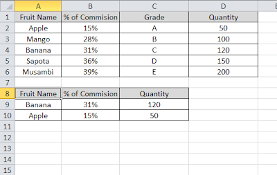
    To make this simple I am taking a small table which has 4 columns for better understanding.  From there we need to fetch only second column data and the 4 th column data.
    Excel VLOOKUP Tips and Tricks
    So i am using the VLOOKUP formula as mentioned below.
    =VLOOKUP($A9,$A$1:$D$6,MATCH(B$8,$B$1:$D$1,1)+1,FALSE) in column B9 and copy the same in C9, B10 and C10 also. In cell B9 it returns 31% which is the % of Commision of Banana from the table and in C9 it returns 120 which is quantity. Similarly, it returns 15% and 50 in B10 and C10 respectively.
    Explanation on the Above VLOOKUP formula with MATCH function:
    The lookup value column is made constant and the data range both rows and columns made constant. So where ever we paste the data, the lookup range should be the same and lookup value will be on the same column but it may be in different rows as we are not made row index constant.
    The third argument of vlookup,  ‘index_number’ which refers to the column from where vlookup should fetch the data, we have used MATCH  function. The MATCH function searches for a specified item in a range of cells, and then returns the relative position of that item in the range. In our example, match function returns relative position of the required column header in the headers of the our main database headers. The MATCH function position number starts from 0 and VLOOKUP starts with 1. So we are adding 1 to the relative position returned by MATCH function.
    As I said earlier, this is the one of  simple yet very useful combination of  formulas in a real time excel profession. I have faced many situation in my professional life, where it takes a huge time if we use classic vlookup function to fetch few data from a huge database. This saves our precious time also accuracy as there is very less chances for the error. Do let me know, if this Excel tip helpful for you and also if you face any problem using this tip.