Nokia Lumia 620 is the most affordable Windows 8 phone as of now. Though it got delayed to enter the Indian market, it is making news for its performance for the price it is offered. The latest Lumia 620 price in India is ₹14400. Before looking into the advantages and Disadvantages of Lumia 620, let us have a quick look into the features of Lumia 620.

To Start with Nokia Lumia 620 comes with 3.8 inch ClearBlack display screen with a screen resolution of 800*480 pixels which makes 246 ppi pixel density. Interms of numbers it is not spectacular. But it offers very good sunlight legibility and wide viewing angles. Colors are vivid and images looks sharp.Considering the price of Lumia 620, there is no phone has such a decent display from any of the well established brands.
Nokia Lumua 620 comes with a 1GHz dual core Krait processor with 512MB of RAM and Adreno 305GPU. For storage it offers 8GB on board storage, 7GB SkyDrive Space and support for micro SD card support upto 64GB. For connectivity, device has 2G, 3G, Dual band Wi-Fi, Bluetooth 3.0, NFC and microUSB 2.0. There is 1300 mAh battery which powers the phone is capable to hold the battery life a full day with normal use.

Nokia Lumia 620 Camera is another plus point. It has got 5MP primary camera with LED flash which can record 720p HD videos at 30fps. You cannot compare the quality of the Lumia 620 camera with high end phones. The low light performance is just average. Having said that, it is capable of recording 720p HD videos unlike other similar priced phones which provides only 420p videos such as Samsung Galaxy S Duos which is slightly priced higher than this model. The Nokia Lumia 620 also features a front facing camera which can be used for Video calling, Video Chat and Self portraits. Now let us look into the some of the key disadvantages of Lumia 620.
Disadvantages of Nokia Lumia 620:
Lack of ample Apps: The Windows Phone 8 does not have as many apps as compared to iOS and Android. Also, it is observed that, some of the apps and games such as Angry bird is available only in paid version. The number of apps count is increased but there is no match compared to Android and iOS. It is not a big deal if you are a casual gamer.
Below average low light camera performance: As mentioned above, the snaps taken in the indoors with low light conditions, looks very soft. There is a lot grains.
Complicated SIM card slot: The sim card slot in Nokia Lumia 620 is not placed conveniently. It takes a bit of understanding before inserting the SIM. It could have better, if Nokia made it simple.
Advantages of Nokia Lumia 620:
Powerful processor: It has got the 1GHz dual core Krait processor which makes phone to run apps and games smoothly. Even the HD video play back is good.
Good Display Screen: The Lumia 620 has got very decent display screen. With its ClearBlack technology, the outdoor readability is very good.
Pre installed Nokia Apps: Nokia Lumia 620 stands apart from other Windows phones because of its Nokia propriety apps. For example, the Nokia maps or HERE maps provides outstanding offline navigation system. The City lense app shows the nearest worth visiting places. There are many apps like this but mentioned few.
Ability to Play vast media formats: Nokia Lumia 620 plays full HD videos and all formats including MOV and AVI were natively supported by the phone. Even playing the audio and video from the SD card also very smooth.
Summary: There is no phone is perfect and each phone has its downsides. Nokia Lumia 620 also no exception to it. It all depends on the budget of ours and the features we are looking for. Some of the features looks interesting but not useful on day to day life and we use very rarely like the Smart Stay feature in Galaxy S4. In my opinion, Nokia Lumia 620 is a great phone for the price it is offered if you are looking for a phone which is good for making and receiving calls, playing casual games and using it as navigation tool. You can read more detailed info on this in Nokia Lumia 620 Review.
Author: Aniruddh
-
Nokia Lumia 620 Advantages and Disadvantages
-
Creating a Calculated Field in Excel PivotTable
In the last post on Excel PivotTable, we have seen how to create a PivotTable. Here we will see how to add a new field called calculated fields. Calculated field in PivotTable can be created by performing simple arithmetic calculation on existing field.
Steps to Create a Calculated Field in Excel PivotTable:
- Click any Field in the pivot Table. The PivotTable Tools become available.
- Click on ‘Options’ and then Click on Field list( In Excel 2010, it is ‘Fields, Items,&Sets.
- Click on Formulas. A Menu appears.
- Click calculated Field. The insert Calaculated Field dialog box appears.
- Type the name for the new field
- Double click an existing field to use in defining the field
- Type the operator and the value or the filed such as *1.5
- Click on Ok.
Values of the calculated field fill the data area and the calculated field appears at the end of the field list.
-
Excel Pivottable Quick Tips and Tricks
Using Excel, we can keep the track of our data in different ways and we can perform calculations. It will be useful for analyzing the data and thus understand it better and to make better decision. In post will give you an idea on what is pivot table and how to create pivot table in Excel.
Excel PivotTable is one of the most useful tool and sadly least understood tool also. Like cross tabulation in statistics, a PivotTable show how data is distributed across categories. For example, you can analyse data and display how different products sell by region and by quarter. Alternately, you can analyse income distribution and consumer preference by gender and age bracket. Excel PivotTable answers very useful questions on the data. Let us start with how to create PivotTable in Excel.
Creating PivotTable in Excel:
Step1: Select the data on which you want to include in the PivotTable.
Step2: Click on Insert Tab
Step3: Click PivotTable. The Create PivotTable dialog box appears.
Step 4: Click a data source. If you already selected a range in the current workbook, the range appears here. Just verify the data range selected covered all the data points.
Step 5: Click to select where to place report. If you want to place the report in the existing worksheet, type the location.
Step 6: Click Ok. Now you will see the PivotTable Field list.
Step 7: We need to place elements in a way that we need the data to be presented. So let us have quick overview on the PivotTable Layout.
PivotTable layout consist of several elements: Report Filter, data, columns and rows. You can use the PivotTable Field list to organize these elements, When working with the PivotTable, you can bring the Field List into view by clicking anywhere in the PivotTable, then click the Options Tab and then clicking Field List. Report Fields enables you to filter the data that appears in your report. Row fields appear as row labels down the left side of your PivotTable and Column fields appear as Column lables across the top of your PivotTable. You place your continuous data field in the Value box. Field placed in the Values box make up the data area. You can also arrange and rearrange field layouts.
Step 8: Click to select the fields you want to include in your PivotTable.
Step 9: Click and Drag fields among the report, Column,Row Lab and Value boxes.
Step 10: Click on the field header and then choose your sort and filter options. -
Using Formulas in Excel using Named Ranges
Constructing the formulas sometimes very complicated especially when you use several functions in the same formula or multiple argument for a single function. For this, if you use named ranges or constants which refers to a frequently used value or constant. A ‘Named range’ is a name you assign to a group of related cells. Using named constants and named ranges can make creating formulas and functions easier by enabling the use of names that clearly identify a value or range of values. The named ranges or named values also helps you to understand the formula to other easier. Let us have a look into how to define a named ranges and values in excel and how to use them in Excel formulas.
Defining Named Ranges and Values in Excel

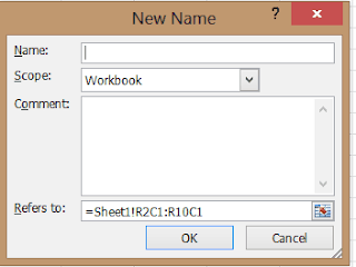
- Click on the Formula Tab and then Click on ‘Define Name’. The new name dialog box appears.
- Type the name you want to assign it to a range or constant. Ideally, it will be good practice to give a name which related to the value it refers to, though you can name it whatever you want.
- Select the scope of the defined name. You can choose for the full workbook or specified sheet.
- In the comment section, you can write something which describes your Named range or value. It is optional. It is better to write as it will be helpful when you refer this range after some time as you might forget what it refers to.
- ‘Refers to’ section you can enter a constant value or a range of cells. You can use browse icon to select the ranges or even you can manually enter it.
- Click Ok. You are done with defining the Names Range or Value.
Creating the Formulas using defined Named Ranges
We have already defined the range with a name. Now we will how to use that in the Excel functions or formulas. Use the functions or Formulas as usual. But instead of writing the range, type the name of that range you have defined. Below is the simple example which will give you better idea on how to use Named ranges in Excel Formulas.
Below is the Sample Excel data which has Smartphone names and its price.

Here I have defined the range from B2 to B5 as ‘PriceRange’. Now for using this range in SUM function look as mentioned below.
=SUM(PriceRange).
Note: When you are using the named range in Excel Formula, as soon as you type first letter of your named range, you will see a drop down list which shows the named ranges. You can use that for easy to type the names.
-
Windows 8 Keyboard Shortcut Keys
Windows 8 the latest operating system from Microsoft is made big news because of its new User interface. This operating system is mainly built to use on touch screen devices. However, it runs and functions properly on even on normal non touch screen laptops and desktops. Those who are familiar with older versions of Windows, feel little difficult to adopt. So here is a simple tricks using keyboard shortcut keys to make life easier on Windows 8.Windows 8 Keyboard Shortcut Keys:
1. Windows Key+C: This brings the side bar menu. Alternatively, you can move the cursor to right bottom or top corner to get this menu.
2. Windows Key+I: This will show you the quick settings menu in the right side. Using this menu provides access to Control panel, brightness of the screen, Power options, Volume etc. This is one of the most handy shortcut key and it is very useful for me because I do not have the touch screen device.
3.Windows Key+D: This shows the desktop. It works even if you are in modern UI page or any other pages are open and if you want to go back to desktop, you can use this shortcut key.
4. Windows Key: This will bring the modern UI.
5. Windows Key+.(Period): This will snap the active app to right side bar. For example, you might have opened news app and you want to open other things. You can keep that modern UI app in the right side, so that even if you are opened other software or app, the side bar shows the your modern UI app.
6. Windows Key+X: This gives you the power menu through which you can access Device manager, Run command, Disk Management etc.
7. Windows Key+E: This quickly takes you to the My computer screen. This is another very useful shortcut key in Windows 8. Because there is no direct shortcut key to My computer in Windows 8 like its predecessors.
8. Windows Key+Q: This shows the page which shows all the apps installed on the system
9. Windows Key+F: You can this shortcut key to search for an app
10. Windows Key+R: This opens the run commandOther Miscellaneous Shortcut Keys For Various Tasks:
1. For shutting down or restarting the system: Press Windows Key+I. This brings the right side settings menu. Choose power and select shutdown or restart.
2. For showing the system information: Windows Key+X. This brings the power menu options in the left bottom corner. In that select the ‘System’. The new page opens which shows the system information such as Processor, RAM etc.
3. Switching between pages or apps: Press Alt+Tab: using these two keys you can toggle between the active applications or pages. Use Alt+Tab+Shift to select the applications in the backward directions.
4. Typing Indian Rupee Symbol: You can use Shit+Ctrl+$: This writes the rupee symbol if you are enabled the Indian keyboard layout. I have written a detailed post on how i enabled rupee symbol on my Windows system You can read on this here . It works on all the keyboards irrespective of whether rupee symbol is written in the keyboard or not.