Author: Aniruddh

  • Excel Formula to return the last nonblank cell in a column or Row

    Some times in Excel worksheet which we update frequently by adding new data to its columns and we need to reference the last value in a particular column. That is the value most frequently entered. We can achieve this combining two excel worksheet formulas COUNTA and INDEX. The source of this tips is John Walkenbach’s Excel 2010 Tips &Tricks book. To learn about find the last row using Excel VBA click here.

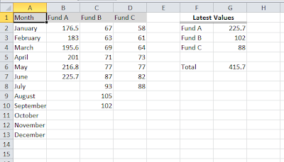
    Below is the simple example with a excel worksheet which tracks the value of three funds in columns B to D. The data updates each and every month. The motto is to get the latest value for each fund and add the values of this.These value will be updated in the cells G2:G4.

    Returning last Columns value in Excel
    The Excel formula used in G2,G3,G4 are as follows.
    =INDEX(B:B,COUNTA(B:B))
    =INDEX(C:C,COUNTA(C:C))
    =INDEX(D:D,COUNTA(D:D))

    Explanation on how this Excel Formula works: The COUNTA worksheet formula used above counts the number of non empty cells in the selected Column.Then this value is used as the second argument for INDEX worksheet function.  In the the first formula, in column B the last value is in row 6 hence COUNTA returns 6  and the INDEX function returns the 6th value in the column.

    The above formula works on most of the situations. However, if the column has one or more empty cells interspersed(Empty cell in between the cells which has values), determining the last nonblank cells is challenging as COUNTA function doesnot count the empty cells.
    The following array formula returns the content of the last non empty cell in the first 1000 rows of column C, even if column C contains blank cells.
    =INDEX(C1:C1000,MAX(ROW(C1:C1000)*(C1:C1000<>””)))
    Note: As this is a Array formula of Excel, you need to press Ctrl+Shift+Enter instead of just Enter. Otherwise it given wrong output.
    You can change the formula to work with a column other than column C. To use a different column, change the column reference from C to whatever column you need. If the last non empty cell occurs in a row beyond row 1000, you need to change the two instances of 1000 to a desired row number. The fewer rows referenced in the formula, the faster the calculation speed.
    To return the last non empty cell in a row, you need to use following excel array formula. It works similar to above formula, but finds last row instead of last column(In this example, row 1.
    =INDEX(1:1,MAX(COLUMN(1:1)*(1:1<>””)))
    to use this formula for a different row, change the the three 1:1 row references to correspond to the correct row number.

  • How to Perform two column Lookup on Excel

    The VLOOKUP function in excel does not handle multiple criteria by default. However, with little tweaking the source data or with the help array formula we can perform multi condition lookup. In this post, we will learn the way to do two column lookup on Excel.

    Let us take a sample data.

    Perform two column Lookup on Excel

    To make this formula we have defined user named ranges.

    Range(C4:D6) is named as lookup_Table

    Other related posts:

    VLOOKUP in EXCEL Tips and Tricks

    ROW and Column VLOOKUP

    Perform two column multi condition vlookup using the helper column

    As VLOOKUP does not take multiple criteria, we need to insert a new column called helper Column. In this column we need to concatenate the fields of two column. In our example, we have concatenated Brand and Model using the formula concatenate or with the help of “& “.

    Formula in cell C4 is

    =A4&B4

    Final vlookup formula is

    =VLOOKUP(G3&G4,lookup_Table,2,FALSE)

    How this conditional vlookup works

    In the example, we want to lookup price using vlookup based on brand and model.

    One of the limitation of VLOOKUP is it handles only one condition. The lookup value will be searched in first column of the selected data range. To overcome this limitation, we are using the helper column.

    In the helper column, we have concatenated the Brand and model. The lookup value also we have joined together. In the example, VLOOKUP searches for BajajPulsor in the range C4 to C16. It is there in 9 the row. Now it will return the corresponding value in 2nd column. That is 53000.

  • Excel formula to count the Characters in cell based on different criteria

    There is a direct Excel formula to count the number of characters in a cell. However, we sometimes come under a situation where we need to count a specific character in a cell or an occurrence of a substring in a cell.  Here are the steps to achieve these requirements.

    Counting all the characters in a Cell

    To count the number of characters in a cell, there is an Excel function called LEN. 

    Syntax of LEN function

    =LEN(text)

    Examples for using Excel LEN function:

    =LEN(A1)- it counts the number of character in Cell A1

    =LEN(“Apple”)- counts the number of characters in the word “Apple”

    Counting a specific characters in a Cell

    To count a specific character in a cell, we need to use substitute and upper functions along with LEN function.

    Example:

    Let us consider we have a word “Apple” in Range A1 and we need to calculate the number of instances of “P”.

    =LEN(A1)-LEN(SUBSTITUTE(UPPER(A1),”P”,””)) which returns 2.

    This formula calculates the number of instances of “P” irrespective of case. If you want this formula to be case sensitive then formula becomes as mentioned below.

     =LEN(A1)-LEN(SUBSTITUTE(A1,”p”,””))

    Explanation:

    The Formula counts the total number of characters in the cell and subtracts the count of character of the cell excluding the character we need to calculate the count. Here SUBSTITUTE function is used to exclude the character “P”. SUBSTITUTE function is case sensitive; hence we have used “UPPER” function which makes all the characters in the cell to upper case in the first example. 

    Counting the occurrences of a substring in a cell

    Below example demonstrates on how to calculate the count of a specified string(more than a character) in a cell. 

    =(LEN(A1)-LEN(SUBSTITUTE(UPPER(A1),UPPER(B1),””)))/LEN(B1)

    In this example, the main string is in Cell A1 and the substring which we need to count is in cell B1.  For example. Cell A1 contains “Excel to Excel” and B1 contains “Excel” then the result is 2. The formula is not case sensitive. If you want to the formula to be case sensitive, then remove UPPER function which looks like below.

    =(LEN(A1)-LEN(SUBSTITUTE(A1,B1,””)))/LEN(B1).

  • Different ways of using Single Criterion SUM function in Excel

    We have already seen the basic syntax and how to use single criteria SUM in Excel. In this post, we will see how use conditional sum based on difference scenarios. For detailed explanation on SUMIF function please read here.
    Examples for Using conditional sum Excel Function SUMIF: Below are the some of the Excel example based on different situations.

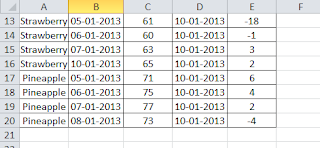
    Conditional sum Sample data
    Sample Data

    1. Summing only Negative OR Positive values using Excel SUMIF Function:

    The below formula will add the “difference” column values whichever is less than zero.
    =SUMIF(E2:E20,”
    Similarly you can add the values with positive value.
    =SUMIF(E2:E20,”>0″)

    Now if we want to find the total variations, we need to sum all negative values and positive values. Below is the formula to find total sum considering absolute values.
    =ABS(SUMIF(E2:E20,”0″) which returns 86. Here we did calculate the sum of both negative and positive values and then added these two making negative values absolute. 

    Note: The SUMIF function can use three arguments. However it is not mandatory to use third argument. If we omit the third argument, then Excel adds the values in the 1st argument when the criteria is met.

    2. Summing values based on a different Range:  For this we need to use the third argument of SUMIF functions.  As we know, first argument is the range which should be matched with the criteria(argument 2) and the third argument is the range which should be added when given criteria is met. Following SUMIF formula demonstrates the same.
    =SUMIF(E2:E20,”>0″,C2:C20) which returns 940. In this example, excel adds the “price” where the difference has positive value(Greater than Zero).
    3. Summing Values based on a text comparison: Some times we need to compare the text value of a range and then perform SUM.  Following are examples for the same.

    =SUMIF(A2:A20,”Apple”,C2:C20) which returns 444. This formula adds the range “Price” when “Data” Column has the text “Apple”.
    =SUMIF(A2:A20,”<>Apple”,C2:C20) which returns 997.This formula adds the range “Price” when “Data” Column does not contains text “Apple”.

    4. Summing Values based on a date Comparison: We can use Excel SUMIF formula to add the values based on given date criteria. Following is the example for the same.
    =SUMIF(B2:B20,”>=”&DATE(2013,1,7),C2:C20) which returns 790.
    =SUMIF(B2:B20,”>=”&TODAY(),C2:C20) which returns 217.

    Note: As you might have observed, we have used a expression as a second argument which is a criteria. The expression used in first example is DATE and in second it is Today().DATE function returns the date and Today function returns Todays date.  Also the comparison operator, enclosed in a quotation mark is concatenated using & operator with the result of the DATE or TODAY() function.

    Please share your thoughts or queries on these examples and also share any tips for using SUMIF function you might know in the comment section.0>0>

  • Using VLOOKUP on Excel-Explained with Syntax and Examples

    VLOOKUP functions of excel is very useful when you need to return a value from a table or a range of cells by looking up another value. VLOOKUP on excel can be used for finding the value in a range which are present in the other range in the same sheet or other sheet and other excel files. Let is quickly look into the syntax of vlookup function and examples on how to use VLOOKUP on Excel.  Do note than simple VLOOKUP function works with only single criteria. If you are looking for 2 or more criteria vlookup, the please refer my previous post multi criteria vlookup.

    Syntax of Excel VLOOKUP Function:

    = VLOOKUP( value, table_array, index_number, Typeoflookup )
    where
    Value: is the value to search for in the first column of the table_array or range of cells. Value can either a text or a numerical value.
    table_array: is the range of cells where you need to lookup for the value.
    index_number: is the column number in table_array from which the matching value must be returned. A index_number argument of 1 returns the value in the first column in table_array; a index_number of 2 returns the value in the second column in table_array, and so on.
    Typeoflookup: This is not mandatory. However this will chose between exact match and relative match.  If you use TRUE or if you omit this argument, then non exact match lookup will be performed. If this is set to FALSE, then vlookup does the exact match
    Note and Troubleshooting Tips on Excel:
    • If  “Typeoflookup” is either TRUE or omitted, the values in the first column of table_array must be placed in ascending sort order; otherwise, VLOOKUP might not return the correct value.
    • If “Typeoflookup” is FALSE, the values in the first column of table_array do not need to be sorted.
    • Excel vlookup returns #VALUE! if  “index_number” is less than 1 and returns  #REF! if the  “index_number”Greater than the number of columns in table_array. Also one more error value comes with VLOOKUP is #N/A. Excel returns #N/A when there is no exact match or the value you are matching in the range is not found.
    •  If there are two or more values in the first column of table_array that match the lookup_value, the first value found will be returned

    Example on Using VLOOKUP formula in Excel:

    Excel Examples
    Sample data

    Using vlookup with Exact match:

    Considering above sample data, if you need to lookup for the value “Banana” and fetch the Rating, use the formula given below.
    =VLOOKUP(“Banana”,A2:C6,3,FALSE) which returns C.

    Using vlookup with non Exact match:

    This is useful, when you need relative value. Say for example, your matching value based on the “% of commission” and you want to return the ratings. Here do not that, for using non exact match the first column of lookup range  must be placed in ascending sort order.
    =VLOOKUP(33%,B2:C6,2,TRUE) which returns C. Here first instance of nearby value is taken by the formula.

    Formatting the VLOOKUP on Excel using ISNA and IF functions:

    When there is no match found, excel returns #n/a.  This is will give problems when you need to use SUM function on the return value of returned value.To overcome this, we need to use ISERROR function. This very useful, if you are creating a template with VLOOKUP function.

    Examples:
    From the same above sample table, we will match Strawberry. The formula returns #n/a as the match is not found on the table.
    =IFERROR(VLOOKUP(“Strawberry”,A2:C6,3,FALSE),”Not Found”) which   returns “Not found”.
    The IFERROR functions syntax is =IFERROR(Value, value if error) where “value” is the data which needs to checked for error and “value for error” is the value to be returned incase of error.
    In above example we use VLOOKUP return data as value and “Not Found” used if the returned value is #N/A.
    IFERROR function was introduced in Excel 2007. Hence if you are using earlier version of Excel 2007, then you need to use IF function and ISERROR function of Excel. So the formula is as shown below.
    =IF(ISERROR(VLOOKUP(“Strawberry”,A1:C6,3,FALSE)),”Not Found”,VLOOKUP(“Strawberry”,A1:C6,3,FALSE))
    Note: Do not use this function unless you have earlier versions of excel as this will lead to calculation time. This is because for every time you use the function, excel needs to calculate vlookup twice. when range to lookup is more and number of instances of using this formula more, then excel will take really long time to calculate and return the right values.
    Please do share your feedback and tips which you know in the comment section below. If you need any specific support on Excel, then mention your query in comment section, I will try to answer your query.

    Video Tutorial for VLOOKUP