Category: Excel Tips

Excel tutor on formulas, tips and tricks and VBA.

  • EXCEL XLOOKUP Function – Advantages and examples

    XLOOKUP is the latest addition to Excel lookup family of functions. It is much more functional excel formula than VLOOKUP or HLOOKUP. In this post, let us explore all about this new EXCEL XLOOKUP function with Syntax and examples.

    XLOOKUP formula is available only on Office 365 at the time of writing this. It may roll out to other version in the coming months.

    What is XLOOKUP? How it is different from VLOOKUP or HLOOKUP?

    XLOOKUP allows us to search for a value in a range or table and return the matching result. It is similar to VLOOKUP/HLOOKUP but, it offers so much more. For example, VLOOKUP can do only vertical lookup and HLOOKUP will do only horizontal lookup. XLOOKUP can be used for vertical or horizontal lookup. We will explore more on this in our example section.

    XLOOKUP has just 3 mandatory parameters and 3 optional parameters.

    The mandatory parameters are

    1. The value you are looking for.
    2. The list where the value to be searched.
    3. The list where you want the result.

    Advantages of XLOOKUP in EXCEL

    • XLOOKUP is simple and easy to use: You just need to write =XLOOKUP(What you want to find, list where you want to find, result list). You will get the answer. It is less error prone as well. No need to use the index number or define on whether you want to exact or relative match.
    • Supports right to left lookup: By default, this function has support for right to left lookup.
    • IFERROR is built in as parameter: Most of the times, we will wrap VLOOKUP formula with IFERROR to hide the #N/A. However, XLOOKUP has 4th parameter in which you can define the default output if the the value is not found.
    • Reference as output not the value: This means that, you combine XLOOKUP outputs with other formulas to get innovative outputs.

    XLOOKUP Syntax

    Basic formula with mandatory fields

    =XLOOKUP(What you want to find, list where you want to find, result list)

    Optional Parameters

    Only 3 parameters are mandatory for XLOOKUP formula. However, you can use optional 4th, 5th and 6th parameters to explore additional features.

    4th Parameter in XLOOKUP: IF not found: This parameter can be used to define what to do incase if search value is not found. Instead of returning #N/A, you can get your optional output.

    5th Parameter in XLOOKUP: Match Mode or type: By default, match type is exact match. However, you can choose between Exact match or next smaller item or next larger item or Wildcard character match.

    6th Parameter in XLOOKUP-Match direction: By default direction is top down. If you want bottom up, you define it in the 6th parameter.

    XLOOKUP in EXCEL examples

    Let us take the sample data sheet below.

    Example 1: As a alternative to VLOOKUP:

    =XLOOKUP(A2,F2:F10,G2:G10)

    This will look for the value in A2 in the range F2 to F10 and return the corresponding value in the range G2:G10. The result will be “Sales”.

    Example 2: Right to Left Lookup

    One of the advantage with XLOOKUP is right to left lookup. So to get the name, use formula as given below.

    =XLOOKUP(A2,F2:F10,E2:E10)

    This will look for the value in A5 in the range F2 to F10 and return the corresponding value from the range E2 to E10. That is “Jill”.

    Example 3: Lookup bottom up

    When there is a duplicate values in lookup range, you can choose first from the top or first one from the bottom by using the 6 parameter. -1 to bottom first and 1 for top first.

    =XLOOKUP(A8,G2:G10,H2:H10,,,-1)

    This will look for the value in A8 in the range G2 to G10 and return the corresponding value from the range H2 to H10. As we have selected -1 as 6th parameter, it will pick first one from last. The result will be 17-Apr-2020.

    Example 4: Handling Not found error

    In XLOOKUP, you can define what to do incase the search value is not found in the lookup list by entering the 4th parameter.

    =XLOOKUP(A11,F2:F10,E2:E10,”Not Found”)

    This will look for the value in A11 in the range F2 to F10 and return the corresponding value from the range E2 to E10. As the ID “SA104” not available in the range F2 to it will return “Not Found”. You can define any value or a different formula. For example, you can define another XLOOKUP to look for the data in different table as well.
  • Conditional VLOOKUP in Excel with Match Function

    VLOOKUP in Excel is a powerful function. Simple vlookup does search for the value in the left most column in the table and returns the value in the same row from column number provided. If the requirement is to search for both row and column, then we need to use a conditional VLOOKUP in Excel. This needs clubbing of match function with vlookup.

    Recommended Reading:

    VLOOKUP in EXCEL tips and Tricks

    Find matching value in a row and return column name in Excel

    Conditional VLOOKUP in Excel with Match Function

    There are many ways to do conditional VLOOKUP in EXCEL. In this post we will learn one of the simple method to achieve this. For that, we need to use MATCH Excel function.
    By default, we need to enter the column number in the VLOOKUP syntax. To do conditional vlookup which does checks for both row and column, replace column number with match function. The syntax will look like below.
    VLOOKUP( lookup_value, table_array, MATCH (lookup_value, lookup_array, [match_type]), [range_lookup] )

    Explanation on how it works

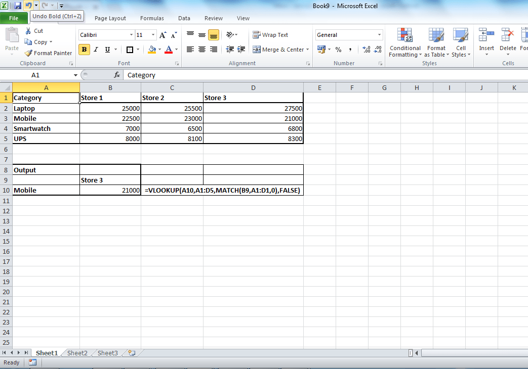
    Lets a take a simple example. Refer the table below. The row has store details and in column has categories. To return corresponding value by matching  both row and column, this conditional vlookup formula will help.

    Conditional VLOOKUP in Excel

    Formula used here is 

    =VLOOKUP(A10,A1:D5,MATCH(B9,A1:D1,0),FALSE)

    In this example, instead of hard coding the column number, we have used match function. MATCH function return the relative position of an item in an array that matches a specified value in a specified order.  In our example it return the column number of the row header Store 3.

    Syntax for Excel MATCH function is

    =MATCH(lookup value, lookup array, [match type])

    This can be achieved through combination of match and index formula too. However, personally for me this is the most convenient way to do row and column vlookup in excel. If you have any specific queries on VLOOKUP in excel, feel free to write to us in the comment section below.

  • Excel Formula to Convert Date To Weekday Name Or Month Name

    How to convert a date to Weekday Name Or Month Name or Year? For example 13-03-2018 to Tuesday or March or 2018. This is one of the most frequently asked queries. So let’s learn an Excel Formula to Convert Date To Weekday Name Or Month Name.

    Recommended Reading

    Excel Tips


    Excel Formula to Convert Date To Weekday Name Or Month Name

    Excel Formula to Convert Date To Weekday Name Or Month Name or Year

    One of the frequently used EXCEL formula to convert date to Weekday Name Or Month Name or year is TEXT Function.

    The syntax of text function in excel

    TEXT( value, format )

    The TEXT excel function is the easiest formula to use for converting Date To Weekday Name Or Month Name. Let’s learn this with an example.

    We have a date in cell A2 has 13-03-2018(Date-Month-Year format)

    Now we will use TEXT Function

    =text(A2, “ddd”) will return “Tue

    =text(A2, “dddd”) will return “Tuesday

    =text(A2, “mmm”) will return “Mar

    =text(A2, “mmmm”) will return “March

    =text(A2, “yyyy”) will return “2018

    =text(A2, “m”) will return “3

    =text(A2, “d”) will return “13

    Summary of the examples mentioned above.

    A2 is the value or the reference to the cell where date is present.

    The second argument of TEXT function accepts format, You can use the format based on your requirement as mentioned below.

    1. “ddd” will return first three characters of the week name.
    2.  “dddd” will return full week name.
    3. “mmm” will return first three letters of the month name.
    4. “mmmm” will return full name of the month.
    5. “yyyy” will return year.

    Using TEXT function to convert Date To Weekday Name Or Month Name ideal in the scenario where you want the result to be shown in the different cell. If you just want to convert to the same cell, then format cell will be the best option.


  • VLOOKUP Tips and Tricks- EXCEL Tutorial

    VLOOKUP in Excel is one of the most powerful and useful function which helps to save our time on many occasions. Some of the situations where VLOOKUP comes in handy are fetching data from other tables, matching two different series, creating one list from multiple related lists etc.  This post is not on how to use VLOOKUP in excel. This post is all about some of the useful tricks which is helpful to use VLOOKUP in excel in an effective way.

    VLOOKUP Tips and Tricks

    1. Using the $ for lookup value and lookup range

    When you are copy and pasting the VLOOKUP in excel to different cells, you might have noticed errors. This happens because while you are pasting the formula, range changes. To avoid this, you can use the absolute range or value. To make the value absolute you should use $ symbol.

    For example, consider an example.

    =vlookup(a2,c2:d5,2,false)

    The above formula is there in cell G2. If you copy and paste the formula in G3, the formula changes to  =vlookup(A3,C3:D6,2,false). If you copy the formula in the cell H2, then formula changes to =vlookup(B3,D2:E6,2,false). To avoid this, we can use $ or it is called absolute reference.  $ makes the row or column absolute. If you use before column name then, the column will become absolute. If you use before row number, then row number will become absolute.  Likewise, if you use $ before column and row number, then both column and row will become absolute. There are different ways to use absolute references in excel depending on the situations. Let’s learn more on this with the same example mentioned above.

    Scenario 1: =VLOOKUP($A$2,$C$3:$D$6,2,false)- In this case, wherever you copy this formula, it will lookup for the value in cell A2 in range C3 to D5 of the active sheet.

    Scenario 2: =VLOOKUP($A2,$C$3:$D$6,2,false)- Here lookup range and column of the lookup value remains constant. However, row number changes depending on where you paste the formula. This can be used when lookup value in there in column A.

    Similarly, you can use the absolute reference for the range as well.

     2. Understanding error values of VLOOKUP

    Majorly, while using VLOOKUP in excel 3 errors values come out. They are #NAME, #N/A and #VALUE.

    What is this means? How to fix it.

    #NAME error in VLOOKUP:  If you get #NAME error, then it means that there is a spelling error in the formula. Please check the syntax and fix it.

    #VALUE error in VLOOKUP: This commonly appears when the column index number is less than the range you have selected. For example, if you have selected the column index number as 5 wherein the range has only 4 columns this error will come. Please check the lookup range and column index to fix this. Another possible cause might be lookup value length is more than 255 characters.   

    #N/A error in VLOOKUP: This is not necessarily an error.  This means that the value you are looking for in the range is not available.  The things you should check are

    • Is lookup value is correct?
    • Are any blank spaces before or after the lookup value? If yes use trim or clean functions to remove spaces.
    • Have you had selected the range where the first column has the value you are looking for lookup value? -If no, select the range such way that, a column on which you are looking for the lookup value should be the first column in the range. The format of the lookup value and lookup range should be same.

    3.  Working with errors

    When the lookup value is not available in lookup range, VLOOKUP gives error #N/A. If you are using the further calculation based on the resulting result, then that also shows as #N/A. To hide this or to make cells look cleaner you can use the formula IFERROR with VLOOKUP. It will look like this IFERROR(VLOOKUP(….), “VALUE to be WRITTEN IN CASE OF ERROR”)).

    4. ROW and COLUMN VLOOKUP or multi conditional VLOOKUP

    We already know that VLOOKUP in EXCEL can be used for fetching data based on the lookup value. But how to use multi conditional VLOOKUP in EXCEL. This means that the resulting data should be matched with both row and column. This can be done with help of MATCH function with VLOOKUP. You need to replace, column index or 3rd argument of VLOOKUP with match function.

    Example for the same is as mentioned below.

    =VLOOKUP($A9,$A$1:$D$6,MATCH(B$8,$B$1:$D$1,1)+1,FALSE)

    You can read more on this here.

    5. Partial match with VLOOKUP

    Making forth argument of VLOOKUP as TRUE will perform partial match. But it has many restrictions. Instead, you can use wildcard characters in VLOOKUP function to perform partial match. Basic wildcard charecter for partial match are,

    “*”: Find any number of characters after or before text. For example, you can use “Te*” to match the text “Text” from a list or *Te to match the text “Forte”.

    “?”: Use a question mark to replace with a character. For example, you can use “?aste” to lookup for the text “Waste” or “Taste”.

    These are the basic yet effective VLOOKUP tips to make your work easier and use this function more effeciently. If you have any queries do write in the comment section below.

  • How to Round a Number to Closest ten in Excel

    Rounding a number in Excel is very easy. There are situation wherein we need to round a number to closest 10 or 100. For example, if we have a number 115 then 120, if we have 112 then 110. For this there is a dedicated function in Excel called MROUND which comes useful for such scenario. Let us learn more about the function MROUND in Excel.

    Syntax of Excel MROUND function

    MROUND(number, multiple)

    Where,

    • Number Required. The value to round.
    • Multiple Required. The multiple to which you want to round number.

    Note: MROUND rounds up, away from zero, if the remainder of dividing number by multiple is greater than or equal to half the value of multiple.

    Example:

    Below are the few useful examples of MROUND in Excel.

    1. Rounding a number to multiples of 10

    =MROUND(112, 10) Rounds 112 to the nearest multiple of 10 which will return 110

    =MROUND(116, 10) Rounds 116 to the nearest multiple of 10 which will return 120

    2. Rounding a number to multiples of 5

    =MROUND(112, 5) Rounds 112 to the nearest multiple of 5 which will return 110.

    =MROUND(116, 5) Rounds 116 to the nearest multiple of 5 which will return 115.

    =MROUND(118, 5) Rounds 118 to the nearest multiple of 5 which will return 120.

    There are other two Excel function which are very similar to this function but with slight change on the functionality.

    1. CEILING(number,significance)

    This will Returns number rounded up, away from zero, to the nearest multiple of significance. For example

    CEILING(112,5) will return 115

    CEILING(112,10) will return 120

    CEILING(115,5) will return 120.

    2.FLOOR(number,significance)

    This will Rounds number down, toward zero, to the nearest multiple of significance.  For example,

    FLOOR(112,5) will return 110

    CEILING(115,10) will return 110.

    So in summary, MROUND Excel function is useful when we need to round number up or down to the nearest multiple. Whereas if you want roundup decimals then ROUNDUP function is useful. For rounding down decimal ROUNDDOWN excel function is useful. Depending on the requirements, these Excel functions will help us to save our time.