Category: Excel Tips

Excel tutor on formulas, tips and tricks and VBA.

How to Create Pie of Pie or Pie of Bar Charts in Excel

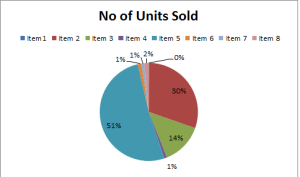
The Pie charts well known for representing size relationship between the parts and entire thing. For example, if a company has multiple units, if you represent the profit of each unit in Pie Charts, it shows profit per unit in percentage. Sum of all slices/units is the total profit of the company. Sometimes, we have the data where some slices are very tiny because of small values which something look like below image. In this scenario pie of Pie or Pie of Bar charts are useful. Let us see how to use Pie of Pie charts in Excel.

How to use Pie of Pie Charts in Excel

Pie of Pie charts in Excel is used to represent separate tiny slices from the main Pie chart and show them in additional Pie charts. Let us see how to Pie of Pie charts in Excel with an example.

1: Select data for which you want to Draw Pie of Pie or Pie of Bar Chart.

2: Go to Insert-> Pie and select Pie of Pie or Pie of Bar Chart.

3: You will get the chart as shown below. Now you can add the data labels to the charts which looks like below.

How to customize Pie of Pie or Pie of Bar Chart

4.By default, Pie of Pie charts in Excel takes some values. You can customize which type of values to moved to the additional chart. For this right click on the chart and choose Format Data Series from the menu.

5. In the Format Data Series dialog, click the drop down list beside Split Series to choose what you want to set the value you want to display in the second pie or bar. You can set Value or Percentage or Position. In this example, I have chosen the less than 10% percentage. The position will be useful if you want to move a specific set of series to second pie.

February 26, 2015
Find matching value in a row and return column name in Excel

When we work in excel sheets, we are required to find a matching value in a row and return the Column name. For example, we need to calculate the lowest priced store from the price table of multiple stores for multiple products. Another example can be found at the primary reason for exits from the exit feedback form analysis. In these cases, even multi-condition vlookup doesn’t help. We will take the first example and find out how to solve this using the Excel formulas.

Recommended Reading:

Conditional VLOOKUP with MATCH In EXCEL
Example:

In the above table we have to return the company name which has lowest price for that product. For this we need to find the column which has the lowest price. So we need to use min(Range) excel worksheet formula. This will give us which is the lowest value. Now we need to find the relative position of the value. For this, match worksheet formula is useful. Now have to get the column name of that position. For this we need to use index function. The final formula will become like below.

=INDEX($B$1:$E$1,MATCH(MIN(B2:E2),B2:E2,0)) which returns Company A.

How it works?

MIN(B2:E2) returns 16999.
MATCH(MIN(B2:E2),B2:E2,0) returns 1
INDEX($B$1:$E$1,MATCH(MIN(B2:E2),B2:E2,0)) returns Company A as column 1 in range B1 to E1 is B1.

Note: The column range for index and match should be the same. Only the row numbers can be different. As match function returns relative position data, the column range should be same for Index function also.

You can tweak this function according to your requirements. You might required to find the column name when you know the exact value in the row. In that case, you need to replace min function with required value.

February 13, 2015
How to Use Checkbox in Excel Worksheet

Checkbox in excel is a very handy tool for creating the checklist or simple user forms. There is no need of any Excel VBA knowledge to insert Checkbox into a excel sheet. This is increase the speed at which user enters data as well as it reduces the chances of misspellings which will give trouble in formulas or pivot tables. So lets start learning how to insert Checkbox in Excel.

Step to Add Check box to Excel Sheet

1. To use Checkbox, you need add it to your ribbon, if it is not already available. To Do this, Go to File->Excel Options->Select Show Developer tab in the Ribbon option if you are using excel 2007. If you are using Excel 201o, then go to File->Options->Customize Ribbon. In the list of main tabs select the Developer check box. Choose Ok to close the Options Dialog Box. This works work well for Excel 2o13 on enabling the developer tab in ribbon.

2. Once Developer Tab is enabled, go to Developer->Selects Chekbox under form controls.

3. Now you can place the Check box where ever you want in your excel sheet.

4. Once you placed the Check-box, left click on your mouse and choose Format Control option.

Format Check Box

5. Go to Control Tab. Here you can choose the default value of the check box whether it is Unchecked or Checked or Mixed. If it is checked the output will true and if it is unchecked the output will be False.

6. The Cell Link refers to the cell on which you want the output to displayed(True or False).

July 13, 2014
How to unhide first row or Column in a Excel Worksheet
At times, in Excel worksheet the first row(Row 1) or first column(column A) doesnot show up. It is tricky to unhide the first row or column as there is no easy way to do it. Based on the situation, you need to apply different method to access the first row or column. So here is the quick possible reasons for hidden first row or first column.
Reasons and Solutions for Hidden First Row or First Column
1. The row or column is hidden: Most of the time we might have hidden that row or column. Unhiding first row or column is as said earlier is not easy. For doing so, simplest method is to select whole sheet and right click and select Unhide.
2. Another possibility is freezed columns or rows: If a excel worksheet has freezed row or columns, then also you will not be able to access some rows and column. Try Unfreezing by going to View->Freeze Panels.
3. Row or Column size reduced to very small: Some excel worksheet which we get has very small sized row or column which we cannot see the row or column. In this scenario, select entire worksheet by selecting entire row. Right click and increase row height. If it is column, then select columns and enter higher column width.
Other solutions for unhiding first row or column:
In the Name Box next to the formula bar, type A1 and then press ENTER.

On the Home tab, in the Editing group, click Find & Select, and then click Go To. In the Reference box, type A1 and then click OK.

Hope these steps helped you to unhide your excel worksheet first row or column. Still if you have any problems share it in the comment section below.
January 27, 2014
How to Remove spaces from a cell in Excel

In today excel tip let us discuss on how to remove leading space and trailing space in a cell of Excel worksheet. By default there are three excel functions which are very useful in removing the space in a cell. The Excel function we are going to use cleanup the cell are CLEAN, TRIM and SUBSTITUTE function.

TRIM Excel Worksheet Function:

The TRIM function is used to remove spaces from a text excluding the one which is there in between two words. The syntax of TRIM function is as follows.

TRIM(text)

Examples:

TRIM(A17) which removes the spaces in the starting of the text and end of the text.

CLEAN Excel Worksheet Function:

The CLEAN worksheet function removes all the non printable characters from the text. In real time, we can use CLEAN function for data which is exported from the other applications which contains characters that may not print with your operating system. The syntax of CLEAN function is as follows.

=CLEAN(text)

If you want to remove non printable characters as well as space, then you need to first use CLEAN function and then use the TRIM function.

SUBSTITUTE Excel Worksheet Function

The substitute function helps you to replace old text with new text. The syntax for substitute function is as follows.

SUBSTITUTE(text,old_text,new_text,instance_num)

Text is the text or the reference to a cell containing text for which you want to substitute characters.

Old_text is the text you want to replace.

New_text is the text you want to replace old_text with.

Instance_num specifies which occurrence of old_text you want to replace with new_text. If you specify instance_num, only that instance of old_text is replaced. Otherwise, every occurrence of old_text in text is changed to new_text.

As you could has assumed, now we can use this formula to replace blank with non blank. Look for the example below.

=SUBSTITUTE(A1,” “,””)

November 27, 2013