Category: Excel Tips

Excel tutor on formulas, tips and tricks and VBA.

Excel Formula to Write Date Format In Excel

In excel we can use a date in different formats according to our wish by clicking on format cells and selecting the required Date format. This works on most of scenarios. But using formula to set the format of date comes handy at times. So in this Excel tips and tricks guide we will learn to use Excel formula which converts date into desired format.

Excel Formula to Convert Date in desired Format

This way of formatting comes very handy when you are using nested function or output of any function which is date. For example you are creating template and sharing with other. They might not be knowing the formatting. So when extend the formula to some other row or column, they will not get the date in desired format. So if you embed the date format in the excel function itself, then it will be more easier. For formating the date in excel using function, text worksheet function is useful. Example is given for such scenario is given in the end of this post.

Syntax of Text worksheet function

=text(Date, Date Format)

Example:
Let us say, the date is in cell A1, then the formula will be
=TEXT(A1,”dd-mmm-yyyy”) which returns date in 24-Apr-2013
=TEXT(A1,”dd-mm-yyyy”) returns date in 24-04-2013 format
=TEXT(A1,”dd-mmmm-yyyy”)return date as 24-April-2013
=TEXT(A1,”yyyy”) returns 2013
=TEXT(A1,”mmmm”) returns April
Hope you got the concept of using Excel formula to get Date format. This Excel formula to format date is very useful when you are using date inside or along with another Formula. For example, let us say in cell A1 we have “todays date” and in cell B1 we have 24-April-2013. When we concatenate these two cells, the result shows todays date41388. To make date to appear in correct formar we need to enter the formula as mentioned below.
=A1&TEXT(B1,”dd-mmm-yyyy”) which returns todays date24-Apr-2013.
Please let me know if you need further details on the same.

April 24, 2013
Excel Vlookup Formula with IF Function-Condition Based vlookup

I have already written on basic vlookup function and conditional vlookup function. In this Excel tutor, i will show you how you can use vlookup function along with IF function. Recently i came across a situation where i need to use different vlookup formula when there is a different scenarios. So i thought even this one will help you also. This excel tips guide will help you on how to perform different range conditional vlookup in excel.

Using VLOOKUP formula with Nested IF function

Actually, i came across this formula, while i was working on a annual salary revision data for a company. There it had all the countries employees with different grades and bands in one sheet. I have been provided with a grid which has increment amount for each grade, grade upgrade and promotion for different countries. The employee data has country details, previous grade, current grade and the band. One way is to split the employee data into three different sheets and performing. But i had a restriction on that. I should do for all countries in one sheet. Below is the steps I have done.

1. I have created one more table for the Proposed Salary increment Grid. A unique id created by concatenating the previous grade, current grade and Band with the help of separating operator !. Please refer the below excel sheet. From A1: F12 contains original data table. From H2: K 12, the calculated salary increments for the different scenarios.
2. Then created the unique code in the employee sheet too with the same logic of concatenating previous grade, current grade and Band with the help of separating operator !. In the example, employee data is in A15 to G21. Added unique code in Column G.
3. Now, in the increment amount field column F17, inserted the vlookup formula with Nested If function as mentioned below.

=IF(B17=”India”,VLOOKUP(G17,$H$4:$I$12,2,FALSE),IF(B17=”US”,VLOOKUP(G17,$H$4:$J$12,3,FALSE),VLOOKUP(G17,$H$4:$K$12,4,FALSE)))

4. Copied the same formula to all the employees. The employee sheet has the increment amount for all the employees based on their grade upgradation or promotion and their countries.

The above logic is simple, Tested the condition and while the condition is met, executed one set of vlookup formula while that condition is not met, tested one more criteria and ran different set of vlookup formula and so on. By default you can Nested if for 7 times. For using IF formula more than 7 times, you need to take help of Excel VBA custom function.

Share your thoughts on the same. If you have any better solution for this or if you need any clarification on this, share it in the comment section below.

April 20, 2013
Using VLOOKUP Formula in Excel effectively using MATCH Worksheet function

In my earlier Excel tutorial post, we have learned how to use vlookup function. In this post, I will show you simple tweak through which you can make VLOOKUP function more effective. This will be useful for you when you want to map huge data.

For example you have base table with more than 20 or 30 columns. From that, you need to fetch selected 5 or 6 columns in different part of the sheet or in different sheet itself. For doing this we need to use MATCH worksheet function along with VLOOKUP function.

Using Excel VLOOKUP with Match Formula:

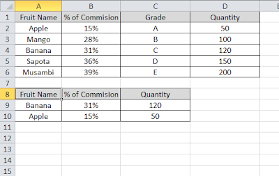
To make this simple I am taking a small table which has 4 columns for better understanding. From there we need to fetch only second column data and the 4 th column data.

So i am using the VLOOKUP formula as mentioned below.
=VLOOKUP($A9,$A$1:$D$6,MATCH(B$8,$B$1:$D$1,1)+1,FALSE) in column B9 and copy the same in C9, B10 and C10 also. In cell B9 it returns 31% which is the % of Commision of Banana from the table and in C9 it returns 120 which is quantity. Similarly, it returns 15% and 50 in B10 and C10 respectively.
Explanation on the Above VLOOKUP formula with MATCH function:
The lookup value column is made constant and the data range both rows and columns made constant. So where ever we paste the data, the lookup range should be the same and lookup value will be on the same column but it may be in different rows as we are not made row index constant.
The third argument of vlookup, ‘index_number’ which refers to the column from where vlookup should fetch the data, we have used MATCH function. The MATCH function searches for a specified item in a range of cells, and then returns the relative position of that item in the range. In our example, match function returns relative position of the required column header in the headers of the our main database headers. The MATCH function position number starts from 0 and VLOOKUP starts with 1. So we are adding 1 to the relative position returned by MATCH function.
As I said earlier, this is the one of simple yet very useful combination of formulas in a real time excel profession. I have faced many situation in my professional life, where it takes a huge time if we use classic vlookup function to fetch few data from a huge database. This saves our precious time also accuracy as there is very less chances for the error. Do let me know, if this Excel tip helpful for you and also if you face any problem using this tip.

April 6, 2013
Creating a Calculated Field in Excel PivotTable
In the last post on Excel PivotTable, we have seen how to create a PivotTable. Here we will see how to add a new field called calculated fields. Calculated field in PivotTable can be created by performing simple arithmetic calculation on existing field.

Steps to Create a Calculated Field in Excel PivotTable:
- Click any Field in the pivot Table. The PivotTable Tools become available.
- Click on ‘Options’ and then Click on Field list( In Excel 2010, it is ‘Fields, Items,&Sets.
- Click on Formulas. A Menu appears.
- Click calculated Field. The insert Calaculated Field dialog box appears.
- Type the name for the new field
- Double click an existing field to use in defining the field
- Type the operator and the value or the filed such as *1.5
- Click on Ok.
Values of the calculated field fill the data area and the calculated field appears at the end of the field list.
February 28, 2013
Excel Pivottable Quick Tips and Tricks

Using Excel, we can keep the track of our data in different ways and we can perform calculations. It will be useful for analyzing the data and thus understand it better and to make better decision. In post will give you an idea on what is pivot table and how to create pivot table in Excel.
Excel PivotTable is one of the most useful tool and sadly least understood tool also. Like cross tabulation in statistics, a PivotTable show how data is distributed across categories. For example, you can analyse data and display how different products sell by region and by quarter. Alternately, you can analyse income distribution and consumer preference by gender and age bracket. Excel PivotTable answers very useful questions on the data. Let us start with how to create PivotTable in Excel.
Creating PivotTable in Excel:

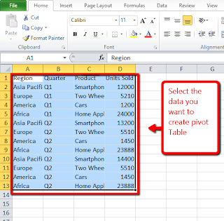
Step1: Select the data on which you want to include in the PivotTable.
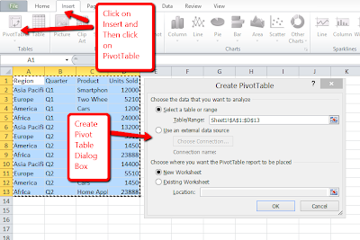
Step2: Click on Insert Tab

Step3: Click PivotTable. The Create PivotTable dialog box appears.
Step 4: Click a data source. If you already selected a range in the current workbook, the range appears here. Just verify the data range selected covered all the data points.
Step 5: Click to select where to place report. If you want to place the report in the existing worksheet, type the location.
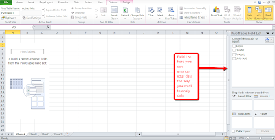
Step 6: Click Ok. Now you will see the PivotTable Field list.
Step 7: We need to place elements in a way that we need the data to be presented. So let us have quick overview on the PivotTable Layout.

PivotTable layout consist of several elements: Report Filter, data, columns and rows. You can use the PivotTable Field list to organize these elements, When working with the PivotTable, you can bring the Field List into view by clicking anywhere in the PivotTable, then click the Options Tab and then clicking Field List. Report Fields enables you to filter the data that appears in your report. Row fields appear as row labels down the left side of your PivotTable and Column fields appear as Column lables across the top of your PivotTable. You place your continuous data field in the Value box. Field placed in the Values box make up the data area. You can also arrange and rearrange field layouts.
Step 8: Click to select the fields you want to include in your PivotTable.
Step 9: Click and Drag fields among the report, Column,Row Lab and Value boxes.
Step 10: Click on the field header and then choose your sort and filter options.

February 24, 2013