Excel inbuilt Average function returns the average(or Mean) of a range of a data. However in many occasions we are required to calculate weighted average. Though Excel do not comes with a straight function to calculate weighted average. This can be done with the use of SUMPRODUCT and SUM functions. Let us start learning about weighted average with an example.
Below is the sample data from a call center and let us calculate the Average Handle Time(AHT) for the day using different intervals calls and AHT. The below data shows that initial hours calls were less and the AHT too was less. But as the call volume increased the AHT also increased.,
The simple average formula =AVERAGE(C3:C9) returns 216.42. The problem with this is that it calculates average without considering the number calls. So we need to calculate average considering the number of calls received on each intervals. Ideally, the weighted average is the appropriate method to calculate like this calculations.
So weighted average formula for the above example is =SUMPRODUCT(C3:C9,B3:B9)/SUM(B3:B9)
This formula multiplies each AHT by its corresponding number calls and then adds all those products. The result is then divided by the number of days. This formula can be easily implemented to other types of calculations where weighted average is required.
There are situations, where we need to use restricted set of data in a list. When in data entry works are carried out by many people, chances are vast that small errors might occur. To overcome this, we can use drop down list in Excel. This not only restricts the user to enter the correct data also it helps to reduce the time to write it manually. So for creating Drop down list, do we need to use Excel VBA feature? No;. Excel provides this feature in the form of data validation. So let us see how to create drop down list in Excel. Steps to Create Drop List in Excel:
Enter the list of items in a range
Select the cell that will contain the drop down list
Choose Data-> Data Tools->Data Validation
In the data validation dialog box, click the settings Tab
In the allow drop-down list select List.
In the source box specify the range that contains the items
Make sure that the In-Cell Drop down option is checked and Click OK
You are done. The drop down list is created in your desired Cell.
Note:
If your list is small, then you can manually enter the list of items in the source box in the Data Validation dialog box.
You can copy paste the Drop down list created cell to other cells to carry the drop down list.
When we apply a formula in Excel which refers to another range or cell, the cell or range reference can be wither relative or absolute. The relative cell reference adjusts to its new location when the formula is copies and pasted in to new cell or range. An Absolute cell reference does not changes even when the formula is copy pasted elsewhere. An Absolute reference is specified with two doller($) signs. For example as mentioned below. Examples for Absolute references: =$C$10 =SUM($A$1:$G$25) Examples for relative references: =C10 =SUM(A1:S25) Normally when we use cell or range references which will be relative references. Excel by default creates relative cell references in formulas except when the formula includes cells in different worksheet or workbook. So where Absolute references are useful? I simple words, this is useful when we need to copy paste the formulas in different cells or ranges.
The formula in the above example table D2 range which multiplies with quantity by the unit price is B2*C2. This formula uses the relative reference. Hence when we copy paste this formula to the next cell D3 it becomes B3*C3. If we use absolute reference in this formula that is instead of B2*C2, D2*$C$2, copying the formula to the below produces incorrect results. The formula in cell D3 is exactly the same as the formula in Cell D2 and returns the total for laptops and not desktops. Now let us use the same tablet to calculate sales tax. The sales tax rate is stored in cell B7. Here formula in Cell E2 is D2*$B$7.
The total is multiplied by the tax rate stored in cell B7. As this is constant for all the items, we need to give absolute references. This reference do not change when we copy the cell. When the same formula in E2 is pasted to Cell E3, the formula becomes D3*$B$7. Here D3 is relative reference hence it changes but B7 remains same.
Excel do not provide a direct way to hide the contents of cells without hiding entire row and column. However there is a indirect way to hide the content in the cell. Hiding cell content comes in handy, if you are using any template.
Steps to hide Cell Content in Excel
There various method to hide cell content in excel without hiding the row or column. These methods just make the content invisible to eye but we can refer this cell using the formulas.
Method 1:Use a special custom number format: Select the cell or cells to be hidden. Go to cell formatting. Select Custom and enter ;;;(three semi colons) in the Type field.
Method 2: Make the font color same as the cell’s background color.
Method 3: Add a shape to your worksheet and position it over the cells or cells to be hidden. Shape color should have same color as the cell background and remove borders.
Method 4: Hiding cell content from in the formula bar
All above method have one shortfall. That is even though content is not seen, it will be seen in the formula bar when cell is selected. To hide the the content from formula bar we need to hide formula bar or perform below mentioned steps .
Select the cell or cells needs to be hidden.
Right click on the cell and go to Format cells. Then click on Protection Tab in the Format Cells dialog box.
Select the Hidden check box and Click OK.
Choose Review->Changes->Protect Sheet.
In the Protect sheet dialog box add a password if you need one. Click OK.
Note: When sheet is protected you can’t change any cells unless cell is unlocked. By Default, all the cells are locked. To unlock cell, select the cells you want to unlock. Go to Format cells and the go to Protection Tab. Uncheck the Locked check box. Tip: Ctrl+1 is the shortcut key to reach format cells dialog box.
Hope this excel tutorial helps. Share your feedback in the comment section below.
There are many instances we need to split a text in a cell. The most common example for this is to split first name and last name. We can perform this using text to column feature of Excel. But if you want to create an template in Excel which requries you to split text in a cell, then you need to use either Excel function or Excel VBA.
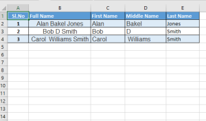
Luckily, Excel provides handy function through which we can extract desired word from the text.The formula uses various text functions to accomplish the task.Each of the techniques used here based on the ‘space’ between the names to identify where to split. So let us take an example of splitting full name into first, middle and last names. Example:
Splitting a text in a cell using Excel Function
Extracting only First name from text using Excel Formula
For extracting first name from full name in cell, we can use left and find functions. So here is the way to how to do it.
Enter the formula in cell C2:
=LEFT(B2,FIND(” “,B2,1))
this will return Alan. similarly same formula in B3 will return Bob. Syntax of Left function:LEFT(text,num_chars)
Where Text is the text string that contains the characters you want to extract. Num_char Specifies the number of characters you want LEFT to extract.
Note: 1.Num_chars must be greater than or equal to zero.2.If num_chars is greater than the length of text, LEFT returns all of text.3.If num_chars is omitted, it is assumed to be 1. Syntax of Find Function: FIND(find_text,within_text,start_num)
Where Find_text is the text you want to find. Within_text is the text containing the text you want to find. Start_num specifies the character at which to start the search. The first character in within_text is character number 1. If you omit start_num, it is assumed to be 1.
Extracting the Last Name from Text using Excel Formula
For extracting last name from a cell in excel, we need to take help of 3 functions. RIGHT, LEN and FIND function.
Eg: in cell E2 enter:
will return Jones. Same formula for the rest the rows. Syntax of Right function: RIGHT(text,num_chars)
Where Text:is the text string containing the characters you want to extract. Num_chars:specifies the number of characters you want RIGHT to extract.
Above functions will not be able to handle any more than two names.If there is also a middle name, the last name formula will be incorrect.To solve the problem you have to use a much longer calculation.
Here is the function to solve this.
Enter =RIGHT(A4,LEN(A4)-FIND(“#”,SUBSTITUTE(A4,” “,”#”,LEN(A4)-LEN(SUBSTITUTE(A4,” “,””))))) in cell B4 will return Smith. Here we have used additional function Substitute Syntax of Substitute function:
SUBSTITUTE(text,old_text,new_text,instance_num)
Where Text: is the text or the reference to a cell containing text for which you want to substitute characters. Old_text: is the text you want to replace. New_text: is the text you want to replace old_text with. Instance_num: specifies which occurrence of old_text you want to replace with new_text. If you specify instance_num, only that instance of old_text is replaced. Otherwise, every occurrence of old_text in text is changed to new_text.
You can use these functions in your excel sheets by making appropriate changes in the column and row numbers. If there is no middle name, the excel function will return #Value.