Category: Excel Tips

Excel tutor on formulas, tips and tricks and VBA.

  • Deleting Constants while keeping formulas in Excel

    In the excel spreadsheet we will have formulas and data values.  There are some situation where we need to delete only values keeping formula in the sheet. Excel provides a solution for this. Here is a quick step by step way to select only values in a cell or only formulas in a cell.

    It is very useful when you are working with excel templates. Excel templates normally will have cells with calculated fields. We just need to update the values. The Excel formulas will automatically generate the calculated cells.  The easiest way to do is just selecting the cells wityh only values and remove it. Now you can enter values in the blank cells. This will protect you from accidental removal of formulas.

    This method of selecting only values in excel worksheet works on all the versions of Excel.  You can use this method to select only formulas or error values in a cell, last cell etc.

    Step to retain only Values and deleting non formula cells

    Below steps will guide you on how to select only values in a excel worksheet.

    Deleting only constants from worksheet

    • Select the range where you want to delete only values, retaining formulas. If you want to delete all non formula value cells on the entire worksheet, then select any single cell.
    • Chose Home->Editing->Find&Select->Go to Special. This will take you to the Go to Special dialog box.
    • In the Go To Special dialog box, select the Constants option and then select Numbers.
    • Click OK. Now only nonformula numeric cells are selected.
    • Press Delete to delete the values.

    Note:

    1. If you need to delete the value cells on a regular basis, then you can specify a name for the input cells. This can be achieved through defining the names to range. After completing Step 4 choose formula ->Defined Names-> Define Name to display the new Name box. Enter a name for the selected cells. Click OK to close the New Name Dialog box and create the name. After naming the input cells, you can select the named cells directly by using the Name box- the drop down list to the left of the Formula bar. Then press delete and you are done.
    2. Shortcut key to reach Goto Special dialog box is Ctrl+G and Alt+S.
  • Working with Time in Excel

    Excel can work with Time very easily. With Time excel can perform many formatting and calculations based time. Let us have a look into this. In this excel tips we will learn few tasks we can perform on Excel with time formats.

    Typing Time in Excel Worksheet

    When time is entered into worksheet it should be entered with a colon between the hour and the minutes, such as 12:30, rather than 12.30.Excel can cope with either the 24hour system or the am/pm system.To use the am/pm system you must enter the am or pm after the time.You must leave a space between the number and the text.
    Example for writing Time in 24 hour format:
    01:30, 2:30, 20:10, 23:30 etc
    Example for writing Time in AM/PM format:
    1:30 AM, 2:30 AM, 8:10 PM, 11:30 PM etc

    Calculation of Time differences in Excel

    :
    You can add or subtract the two times to get know the length of the time or add the two time times to get total time.
    Example for Subtracting two Times in Excel:

    Row/Column A B
    1 Start Time End Time
    2 1:30 AM 2:30 AM
    3 08:00 17:00

    Now you can use formula like this to find difference between the two times.Enter  =A2-B2 in the required result cell. You will get 1:00. And the second one will give you 9:00(A3-B3).
    Example for Adding two times in Excel:

    Consider above table. Adding is very easy. Enter formula =A2+B2 which returns 04:00 and the second row will return 25:00:00. Some time it just returns 1 hours. This is because of the cell formatting. Let us look into the   time formatting.

    Formatting of Time in Excel:
    Considering above example second row 3. Sum goes beyond 24 hours. The general time format will show only the time excluding the number of days. For correcting this,  easiest way is to opt for Custome formatting.
    Applying Custom Formatting to Time to show exact value:
    Time Formatting

    • Click on the cell which needs the format.
    • Choose the Format menu.
    • Choose Cells.
    • Click the Number tag at the top right.
    • Choose Custom.
    • Click inside the Type: box.
    • Type [hh]:mm as the format.
    • Click OK to confirm.hoose Custom.
    • Click inside the Type: box.
    • Type [hh]:mm as the format.
    • Click OK to confirm.
  • Password protecting Excel VBA macros

    We will be facing many circumstance where we need to password protect the excel VBA code we have written. Some times it may be for avoiding unintentional changes to the VBA codes or for hiding our codes from the others. Excel VBA provides a simple way to protect Excel VBA macro using password. This will not only protects from making changes also it protects the code from viewing. Lets start learning on how to password protect Excel VBA codes.

    Step to protect Excel VBA codes using password

    Below are steps to be followed to password protect the VBA codes.

    • First open VBA editor. Shortcut key for opening VBA editor is Alt+F11
    • Go to tools-> Select “VBA project Properties”
    • There new screen pops up. Select “Protection” Tab. You will get a screen similar to given below

    • Select the check box beside “Lock project for viewing” to hide the codes from viewing without password. If you do not want to hide the macro code and just want to protect your codes, then do not select the check box.
    • Enter the desired password in the “Password” labeled text box. Once again type the same password in the “confirmation password field “too.
    • You are done. Save the sheet and close the excel sheet.
    • Next time if you open VBA explorer you will prompted for password to view or modify the codes.

    This is method of password protecting of Excel VBA codes works on almost all current version of Excel.

  • Creating Templates in Excel

    Excel templates are very useful whenever we need to do repeated tasks. Excel VBA does it. But Excel VBA is a little hard to learn and implement.

    Excel templates is nothing but pre defined format. For example if you want to get Agent productivity report in Excel. You have raw reports which has productive hours, non productive hours and other details. Instead of doing every day look up and sum function, create template. That create a new sheet.  In that put all the fiormula or excel functions and required data. So now onwards whenever you need to do the report, just put the raw reports you will get output immediately.

    Advantages of Excel Templates:

    • Saves lot of time
    • Accuracy of the reports increases as manual work is reduced
    • No need to know complicated VB codes.
    • Get time explore new things
    • Do more analysis on data.
    Useful functions and tools to create Excel Templates: Below are minimum Excel formula you should know to create a simple and effective excel templates.
    • Pivot tables: This is one of the tool very useful. You can customize the data the way you want to. Create calculated fields in pivot table to enhance the look and get more data.
    • Vlookup and Hlookup functions: These lookup functions will be very handy while you need to map some fields based on some data criteria. 
    • Conditional sum and count:  Conditional sum function sumif and conditional count function countif are useful when you need to count or sum of the data for a particular data.
    • Multi conditional sum and count: There are many occasions we need to find sum or count based on multiple criteria. SUMIFS, COUNTIFS and sumproduct are the useful functions
    Tips on Creating Excel Templates:
    • Always create a template such a way that, the output of the template matches with desired report format. Do not give a scope for manual work on template on regular basis. This will save time.
    • Use Conditional functions to get ride of error codes such as #n/a.  For this IF function with iserror function will be very useful.
    • While selecting the range, select only the range you have data. Do not select complete sheet. Selecting whole sheet will slow down the template. Using Dynamic ranges will also helpful.
  • Multi Conditional lookup in Excel

    Have you ever came across a situation wherein you wanted to return a value which matches both row and column? VLOOKUP function in Excel returns the value which is matching the row only. In our previous tutorial, we have shown how to perform two column lookup. In this excel tips post, we will guide you on how to perform multi conditional lookup using match and index functions.

    Limitations of Vlookup:

    • VLOOKUP can be used only if the lookup value is in left of the data which we need to extract from the Table or data.
    • VLOOKUP works with one criteria. That is, lookup value is maximum one.

    Multi Conditional lookup in Excel

    To overcome above-mentioned limitations of VLOOKUP, we can use match and index function of excel to get a result like conditional VLOOKUP.

    Using Match and Index function for conditional lookup

    When Match and index functions of excel used together, we can extract the data from a table irrespective of the weather lookup value is left side or right side of the array. So first let us understand Match and Index functions. To perform conditional lookup, we should understand how match and index functions of excel work.

    Excel Index Function

    Excel Index function returns a value or reference from a table or range.

    Syntax of Excel Index Functions:

    =INDEX(array, row_num, [column_num])

    Explanation of Index Function components

    • Array: Is a range or table where we need to extract the data.
    • row_num: In which row the required value is there.
    • [column_num]: In which column the lookup value is present.

    =INDEX(A1:C5,2,3)  returns 3. We are looking for a data which is 2nd row and 3rd column.

    Excel Match Function

    Match function returns relative position of the specified item is a range of cells.

    Match Function Syntax

    MATCH(lookup_value, lookup_array, [match_type])

    • Lookup_value: The value you need to look up.
    • Lookup_Array: The range where you need to search
    • [match_type]: Match_type can be -1, 0, or 1. It tells Excel how to match the lookup_value to values in the lookup_array.
      • 1 — find the largest value less than or equal to lookup_value (the list must be in ascending order)
      • 0 — find the first value exactly equal to lookup_value. Lookup_array (the list can be in any order)
      • -1 — find the smallest value greater than or equal to lookup_value. (the list must be in descending order)

    Note: If match type is omitted, by default excel consider it as 1.

    Example for Excel Match Function

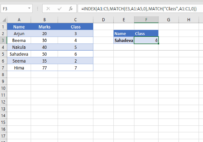
    Consider the same table as above.

    =MATCH(“Sahadeva”,A1:A5,0) returns 5. That is the value “Sahadeva” is in 5th row.

    Using Index and Match together as an alternative to vlookup

    Using index match together will help us in finding 2 criteria lookup and values are present in left of the lookup value.

    Generic Formula

    =INDEX(array, MATCH(lookup_value, lookup_array, [match_type]), MATCH(lookup_value, lookup_array, [match_type]))

    Here what we did is instead of finding row and column numbers we used Match function to find.

    Example:
    =INDEX(A1:C5,MATCH(“Sahadeva”,A1:A5,0),MATCH(“Class”,A1:C1,0)) This returns 6.

    How to MATCH and INDEX work as alternative to VLOOKUP

    We are looking into the table as the range: So, in Index, we used Table as the range. Using Match function, we found rows number of our lookup value “Sahadeva”. For the column number, we once again used Match function to find another criteria column number. That is we are searching for Sahadeva’s Class. So, Class is in 3 row. So, the function returns the value which is in the 5th row and 3rd Column.