Category: VLOOKUP in Excel

VLOOKUP in excel is one of the most useful and powerful function. It helps to retrieve values. VLOOKUP helps to match two series. The list goes big.

Here is the series of posts related to VLOOKUP function in excel. We tried to cover basics to some intermediate level tips. We will be updating new tips and tricks of VLOOKUP in excel regularly.

Proper knowledge of VLOOKUP excel function will ease many of the tasks. It not only simplifies, it also helps to save time.

If you have any queries related to VLOOKUP function in EXCEL feel free to write to us.

  • Conditional VLOOKUP in Excel with Match Function

    VLOOKUP in Excel is a powerful function. Simple vlookup does search for the value in the left most column in the table and returns the value in the same row from column number provided. If the requirement is to search for both row and column, then we need to use a conditional VLOOKUP in Excel. This needs clubbing of match function with vlookup.

    Recommended Reading:

    VLOOKUP in EXCEL tips and Tricks

    Find matching value in a row and return column name in Excel

    Conditional VLOOKUP in Excel with Match Function

    There are many ways to do conditional VLOOKUP in EXCEL. In this post we will learn one of the simple method to achieve this. For that, we need to use MATCH Excel function.
    By default, we need to enter the column number in the VLOOKUP syntax. To do conditional vlookup which does checks for both row and column, replace column number with match function. The syntax will look like below.
    VLOOKUP( lookup_value, table_array, MATCH (lookup_value, lookup_array, [match_type]), [range_lookup] )

    Explanation on how it works

    Lets a take a simple example. Refer the table below. The row has store details and in column has categories. To return corresponding value by matching  both row and column, this conditional vlookup formula will help.

    Conditional VLOOKUP in Excel

    Formula used here is 

    =VLOOKUP(A10,A1:D5,MATCH(B9,A1:D1,0),FALSE)

    In this example, instead of hard coding the column number, we have used match function. MATCH function return the relative position of an item in an array that matches a specified value in a specified order.  In our example it return the column number of the row header Store 3.

    Syntax for Excel MATCH function is

    =MATCH(lookup value, lookup array, [match type])

    This can be achieved through combination of match and index formula too. However, personally for me this is the most convenient way to do row and column vlookup in excel. If you have any specific queries on VLOOKUP in excel, feel free to write to us in the comment section below.

  • VLOOKUP Tips and Tricks- EXCEL Tutorial

    VLOOKUP in Excel is one of the most powerful and useful function which helps to save our time on many occasions. Some of the situations where VLOOKUP comes in handy are fetching data from other tables, matching two different series, creating one list from multiple related lists etc.  This post is not on how to use VLOOKUP in excel. This post is all about some of the useful tricks which is helpful to use VLOOKUP in excel in an effective way.

    VLOOKUP Tips and Tricks

    1. Using the $ for lookup value and lookup range

    When you are copy and pasting the VLOOKUP in excel to different cells, you might have noticed errors. This happens because while you are pasting the formula, range changes. To avoid this, you can use the absolute range or value. To make the value absolute you should use $ symbol.

    For example, consider an example.

    =vlookup(a2,c2:d5,2,false)

    The above formula is there in cell G2. If you copy and paste the formula in G3, the formula changes to  =vlookup(A3,C3:D6,2,false). If you copy the formula in the cell H2, then formula changes to =vlookup(B3,D2:E6,2,false). To avoid this, we can use $ or it is called absolute reference.  $ makes the row or column absolute. If you use before column name then, the column will become absolute. If you use before row number, then row number will become absolute.  Likewise, if you use $ before column and row number, then both column and row will become absolute. There are different ways to use absolute references in excel depending on the situations. Let’s learn more on this with the same example mentioned above.

    Scenario 1: =VLOOKUP($A$2,$C$3:$D$6,2,false)- In this case, wherever you copy this formula, it will lookup for the value in cell A2 in range C3 to D5 of the active sheet.

    Scenario 2: =VLOOKUP($A2,$C$3:$D$6,2,false)- Here lookup range and column of the lookup value remains constant. However, row number changes depending on where you paste the formula. This can be used when lookup value in there in column A.

    Similarly, you can use the absolute reference for the range as well.

     2. Understanding error values of VLOOKUP

    Majorly, while using VLOOKUP in excel 3 errors values come out. They are #NAME, #N/A and #VALUE.

    What is this means? How to fix it.

    #NAME error in VLOOKUP:  If you get #NAME error, then it means that there is a spelling error in the formula. Please check the syntax and fix it.

    #VALUE error in VLOOKUP: This commonly appears when the column index number is less than the range you have selected. For example, if you have selected the column index number as 5 wherein the range has only 4 columns this error will come. Please check the lookup range and column index to fix this. Another possible cause might be lookup value length is more than 255 characters.   

    #N/A error in VLOOKUP: This is not necessarily an error.  This means that the value you are looking for in the range is not available.  The things you should check are

    • Is lookup value is correct?
    • Are any blank spaces before or after the lookup value? If yes use trim or clean functions to remove spaces.
    • Have you had selected the range where the first column has the value you are looking for lookup value? -If no, select the range such way that, a column on which you are looking for the lookup value should be the first column in the range. The format of the lookup value and lookup range should be same.

    3.  Working with errors

    When the lookup value is not available in lookup range, VLOOKUP gives error #N/A. If you are using the further calculation based on the resulting result, then that also shows as #N/A. To hide this or to make cells look cleaner you can use the formula IFERROR with VLOOKUP. It will look like this IFERROR(VLOOKUP(….), “VALUE to be WRITTEN IN CASE OF ERROR”)).

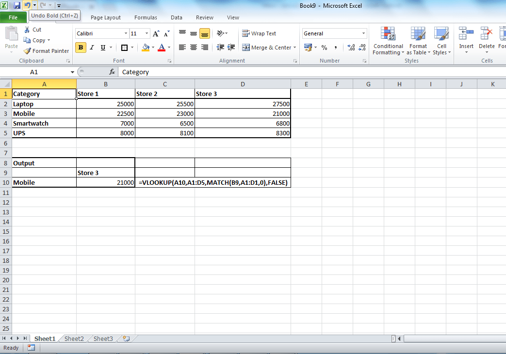
    4. ROW and COLUMN VLOOKUP or multi conditional VLOOKUP

    We already know that VLOOKUP in EXCEL can be used for fetching data based on the lookup value. But how to use multi conditional VLOOKUP in EXCEL. This means that the resulting data should be matched with both row and column. This can be done with help of MATCH function with VLOOKUP. You need to replace, column index or 3rd argument of VLOOKUP with match function.

    Example for the same is as mentioned below.

    =VLOOKUP($A9,$A$1:$D$6,MATCH(B$8,$B$1:$D$1,1)+1,FALSE)

    You can read more on this here.

    5. Partial match with VLOOKUP

    Making forth argument of VLOOKUP as TRUE will perform partial match. But it has many restrictions. Instead, you can use wildcard characters in VLOOKUP function to perform partial match. Basic wildcard charecter for partial match are,

    “*”: Find any number of characters after or before text. For example, you can use “Te*” to match the text “Text” from a list or *Te to match the text “Forte”.

    “?”: Use a question mark to replace with a character. For example, you can use “?aste” to lookup for the text “Waste” or “Taste”.

    These are the basic yet effective VLOOKUP tips to make your work easier and use this function more effeciently. If you have any queries do write in the comment section below.

  • Find matching value in a row and return column name in Excel

    When we work in excel sheets, we are required to find a matching value in a row and return the Column name. For example, we need to calculate the lowest priced store from the price table of multiple stores for multiple products. Another example can be found at the primary reason for exits from the exit feedback form analysis. In these cases, even multi-condition vlookup doesn’t help. We will take the first example and find out how to solve this using the Excel formulas.

    Recommended Reading:

    Conditional VLOOKUP with MATCH In EXCEL
    Example:

    Excel Lookup

    In the above table we have to return the company name which has lowest price for that product. For this we need to find the column which has the lowest price. So we need to use min(Range) excel worksheet formula. This will give us which is the lowest value. Now we need to find the relative position of the value. For this, match worksheet formula is useful. Now have to get the column name of that position. For this we need to use index function. The final formula will become like below.

    =INDEX($B$1:$E$1,MATCH(MIN(B2:E2),B2:E2,0)) which returns Company A.

    How it works?

    MIN(B2:E2) returns 16999.
    MATCH(MIN(B2:E2),B2:E2,0) returns 1
    INDEX($B$1:$E$1,MATCH(MIN(B2:E2),B2:E2,0)) returns Company A as column 1 in range B1 to E1 is B1.

    Note: The column range for index and match should be the same. Only the row numbers can be different. As match function returns relative position data, the column range should be same for Index function also.

    You can tweak this function according to your requirements. You might required to find the column name when you know the exact value in the row. In that case, you need to replace min function with required value.

  • VLOOKUP in Excel Tips and Tricks

    We already learned on how to use VLOOKUP in Excel.  In my earlier different posts, i have shown, the different ways you can use vlookup functions. This post is the summarisation all the things which we have already discussed.

    VLOOKUP in Excel Tips and Tricks

    Here is the list of few VLOOKUP in Excel tips to use the excel worksheet function more effectively.

    1. Use named Ranges:  the vlookup function with normal range variables looks very complicated. To avoid this, use named ranges.  With named ranges, you can do dynamic ranges which saves lot of memory and by that, the time. You can read more dynamic ranges in excel here.
    2. 2 way or conditional vlookup: The default vlookup accepts only single criteria lookup. But using the match function, you use vlookup function which looks for the given value in row as well as in columns. The syntax is same as the normal vlookup apart from inserting match function instead of index number. The match function returns the reference number of the column. To learn more on this read my post on conditional vlookup.
    3. Handling error values in Excel: When the lookup value is not found, vlookup returns, #na. You can remove this by using iferror function. This will make your excel template more clean and easy to perform calculations
    =IFERROR(VLOOKUP(B16,A2:C6,2,FALSE),0)
    4. Use Wildcard characters for related lookup: You can use related lookup using the last argument as TRUE. but, it has a downside. The range should be in ascending order. The wildcard character will help in these situations. Below are the few examples.
    =VLOOKUP(“Galaxy*”,A2:C8,3,FALSE)- returns the value from the range which starts with Galaxy. If there are multiple Galaxy are there, then it will take the first one.
    =VLOOKUP(“????”,A2:C8,3,FALSE) this look for a value with the lookup value length is 4.
    Similarly you can use most of the wildcard characters in vlookup also.

    If you find these tips on VLOOKUP in Excel, or have any queries, feel free to leave feedback in the comment section below.

  • Excel Vlookup Formula with IF Function-Condition Based vlookup

    I have already written on basic vlookup function and conditional vlookup function. In this Excel tutor, i will show you how you can use vlookup function along with IF function. Recently i came across a situation where i need to use different vlookup formula when there is a different scenarios. So i thought even this one will help you also. This excel tips guide will help you on how to perform different range conditional vlookup in excel.

    Using VLOOKUP formula with Nested IF function

    Actually, i came across this formula, while i was working on a annual salary revision data for a company. There it had all the countries employees with different grades and bands in one sheet. I have been provided with a grid which has increment amount for each grade, grade upgrade and promotion for different countries.  The employee data has country details, previous grade, current grade and the band.  One way is to split the employee data into three different sheets and performing. But i had a restriction on that. I should do for all countries in one sheet. Below is the steps I have done.
    Nested IF and Vlookup Formula Example
    1. I have created one more table for the Proposed Salary increment Grid. A unique id created by concatenating the previous grade, current grade and Band with the help of separating operator !. Please refer the below excel sheet. From A1: F12 contains original data table. From H2: K 12, the calculated salary increments for the different scenarios.
    2. Then created the unique code in the employee sheet too with the same logic of concatenating  previous grade, current grade and Band with the help of separating operator !. In the example, employee data is in A15 to G21. Added unique code in Column G.
    3. Now, in the increment amount field column F17, inserted the vlookup formula with Nested If function as mentioned below.

    =IF(B17=”India”,VLOOKUP(G17,$H$4:$I$12,2,FALSE),IF(B17=”US”,VLOOKUP(G17,$H$4:$J$12,3,FALSE),VLOOKUP(G17,$H$4:$K$12,4,FALSE)))

    4. Copied the same  formula to all the employees. The employee sheet has the increment amount for all the employees based on their grade upgradation or promotion and their countries.

    The above logic is simple, Tested the condition and while the condition is met, executed one set of vlookup formula while that condition is not met, tested one more criteria and ran different set of vlookup formula and so on.  By default you can Nested if for 7 times. For using IF formula more than 7 times, you need to take help of Excel VBA custom function.

    Share your thoughts on the same. If you have any better solution for this or if you need any clarification on this, share it in the comment section below.