Multi Conditional lookup in Excel

Have you ever came across a situation wherein you wanted to return a value which matches both row and column? VLOOKUP function in Excel returns the value which is matching the row only. In our previous tutorial, we have shown how to perform two column lookup. In this excel tips post, we will guide you on how to perform multi conditional lookup using match and index functions.

Limitations of Vlookup:

• VLOOKUP can be used only if the lookup value is in left of the data which we need to extract from the Table or data.
• VLOOKUP works with one criteria. That is, lookup value is maximum one.

Multi Conditional lookup in Excel

To overcome above-mentioned limitations of VLOOKUP, we can use match and index function of excel to get a result like conditional VLOOKUP.

Using Match and Index function for conditional lookup

When Match and index functions of excel used together, we can extract the data from a table irrespective of the weather lookup value is left side or right side of the array. So first let us understand Match and Index functions. To perform conditional lookup, we should understand how match and index functions of excel work.

Excel Index Function

Excel Index function returns a value or reference from a table or range.

Syntax of Excel Index Functions:

=INDEX(array, row_num, [column_num])

Explanation of Index Function components

• Array: Is a range or table where we need to extract the data.
• row_num: In which row the required value is there.
• [column_num]: In which column the lookup value is present.

=INDEX(A1:C5,2,3)  returns 3. We are looking for a data which is 2nd row and 3rd column.

Excel Match Function

Match function returns relative position of the specified item is a range of cells.

Match Function Syntax

MATCH(lookup_value, lookup_array, [match_type])

• Lookup_value: The value you need to look up.
• Lookup_Array: The range where you need to search
• [match_type]: Match_type can be -1, 0, or 1. It tells Excel how to match the lookup_value to values in the lookup_array.
  • 1 — find the largest value less than or equal to lookup_value (the list must be in ascending order)
  • 0 — find the first value exactly equal to lookup_value. Lookup_array (the list can be in any order)
  • -1 — find the smallest value greater than or equal to lookup_value. (the list must be in descending order)

Note: If match type is omitted, by default excel consider it as 1.

Example for Excel Match Function

Consider the same table as above.

=MATCH(“Sahadeva”,A1:A5,0) returns 5. That is the value “Sahadeva” is in 5th row.

Using Index and Match together as an alternative to vlookup

Using index match together will help us in finding 2 criteria lookup and values are present in left of the lookup value.

Generic Formula

=INDEX(array, MATCH(lookup_value, lookup_array, [match_type]), MATCH(lookup_value, lookup_array, [match_type]))

Here what we did is instead of finding row and column numbers we used Match function to find.

Example:
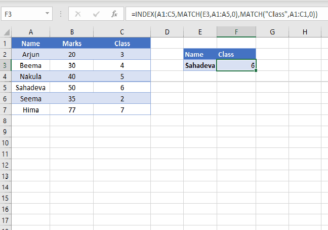
=INDEX(A1:C5,MATCH(“Sahadeva”,A1:A5,0),MATCH(“Class”,A1:C1,0)) This returns 6.

How to MATCH and INDEX work as alternative to VLOOKUP

We are looking into the table as the range: So, in Index, we used Table as the range. Using Match function, we found rows number of our lookup value “Sahadeva”. For the column number, we once again used Match function to find another criteria column number. That is we are searching for Sahadeva’s Class. So, Class is in 3 row. So, the function returns the value which is in the 5th row and 3rd Column.