Tag: Conditional VLOOKUP in Excel

  • Conditional VLOOKUP in Excel with Match Function

    VLOOKUP in Excel is a powerful function. Simple vlookup does search for the value in the left most column in the table and returns the value in the same row from column number provided. If the requirement is to search for both row and column, then we need to use a conditional VLOOKUP in Excel. This needs clubbing of match function with vlookup.

    Recommended Reading:

    VLOOKUP in EXCEL tips and Tricks

    Find matching value in a row and return column name in Excel

    Conditional VLOOKUP in Excel with Match Function

    There are many ways to do conditional VLOOKUP in EXCEL. In this post we will learn one of the simple method to achieve this. For that, we need to use MATCH Excel function.
    By default, we need to enter the column number in the VLOOKUP syntax. To do conditional vlookup which does checks for both row and column, replace column number with match function. The syntax will look like below.
    VLOOKUP( lookup_value, table_array, MATCH (lookup_value, lookup_array, [match_type]), [range_lookup] )

    Explanation on how it works

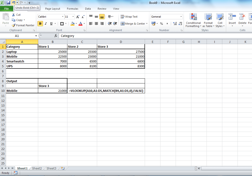
    Lets a take a simple example. Refer the table below. The row has store details and in column has categories. To return corresponding value by matching  both row and column, this conditional vlookup formula will help.

    Conditional VLOOKUP in Excel

    Formula used here is 

    =VLOOKUP(A10,A1:D5,MATCH(B9,A1:D1,0),FALSE)

    In this example, instead of hard coding the column number, we have used match function. MATCH function return the relative position of an item in an array that matches a specified value in a specified order.  In our example it return the column number of the row header Store 3.

    Syntax for Excel MATCH function is

    =MATCH(lookup value, lookup array, [match type])

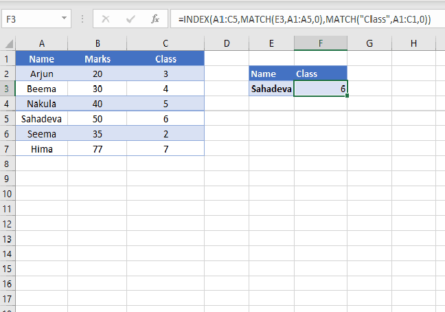
    This can be achieved through combination of match and index formula too. However, personally for me this is the most convenient way to do row and column vlookup in excel. If you have any specific queries on VLOOKUP in excel, feel free to write to us in the comment section below.

  • Using VLOOKUP on Excel-Explained with Syntax and Examples

    VLOOKUP functions of excel is very useful when you need to return a value from a table or a range of cells by looking up another value. VLOOKUP on excel can be used for finding the value in a range which are present in the other range in the same sheet or other sheet and other excel files. Let is quickly look into the syntax of vlookup function and examples on how to use VLOOKUP on Excel.  Do note than simple VLOOKUP function works with only single criteria. If you are looking for 2 or more criteria vlookup, the please refer my previous post multi criteria vlookup.

    Syntax of Excel VLOOKUP Function:

    = VLOOKUP( value, table_array, index_number, Typeoflookup )
    where
    Value: is the value to search for in the first column of the table_array or range of cells. Value can either a text or a numerical value.
    table_array: is the range of cells where you need to lookup for the value.
    index_number: is the column number in table_array from which the matching value must be returned. A index_number argument of 1 returns the value in the first column in table_array; a index_number of 2 returns the value in the second column in table_array, and so on.
    Typeoflookup: This is not mandatory. However this will chose between exact match and relative match.  If you use TRUE or if you omit this argument, then non exact match lookup will be performed. If this is set to FALSE, then vlookup does the exact match
    Note and Troubleshooting Tips on Excel:
    • If  “Typeoflookup” is either TRUE or omitted, the values in the first column of table_array must be placed in ascending sort order; otherwise, VLOOKUP might not return the correct value.
    • If “Typeoflookup” is FALSE, the values in the first column of table_array do not need to be sorted.
    • Excel vlookup returns #VALUE! if  “index_number” is less than 1 and returns  #REF! if the  “index_number”Greater than the number of columns in table_array. Also one more error value comes with VLOOKUP is #N/A. Excel returns #N/A when there is no exact match or the value you are matching in the range is not found.
    •  If there are two or more values in the first column of table_array that match the lookup_value, the first value found will be returned

    Example on Using VLOOKUP formula in Excel:

    Excel Examples
    Sample data

    Using vlookup with Exact match:

    Considering above sample data, if you need to lookup for the value “Banana” and fetch the Rating, use the formula given below.
    =VLOOKUP(“Banana”,A2:C6,3,FALSE) which returns C.

    Using vlookup with non Exact match:

    This is useful, when you need relative value. Say for example, your matching value based on the “% of commission” and you want to return the ratings. Here do not that, for using non exact match the first column of lookup range  must be placed in ascending sort order.
    =VLOOKUP(33%,B2:C6,2,TRUE) which returns C. Here first instance of nearby value is taken by the formula.

    Formatting the VLOOKUP on Excel using ISNA and IF functions:

    When there is no match found, excel returns #n/a.  This is will give problems when you need to use SUM function on the return value of returned value.To overcome this, we need to use ISERROR function. This very useful, if you are creating a template with VLOOKUP function.

    Examples:
    From the same above sample table, we will match Strawberry. The formula returns #n/a as the match is not found on the table.
    =IFERROR(VLOOKUP(“Strawberry”,A2:C6,3,FALSE),”Not Found”) which   returns “Not found”.
    The IFERROR functions syntax is =IFERROR(Value, value if error) where “value” is the data which needs to checked for error and “value for error” is the value to be returned incase of error.
    In above example we use VLOOKUP return data as value and “Not Found” used if the returned value is #N/A.
    IFERROR function was introduced in Excel 2007. Hence if you are using earlier version of Excel 2007, then you need to use IF function and ISERROR function of Excel. So the formula is as shown below.
    =IF(ISERROR(VLOOKUP(“Strawberry”,A1:C6,3,FALSE)),”Not Found”,VLOOKUP(“Strawberry”,A1:C6,3,FALSE))
    Note: Do not use this function unless you have earlier versions of excel as this will lead to calculation time. This is because for every time you use the function, excel needs to calculate vlookup twice. when range to lookup is more and number of instances of using this formula more, then excel will take really long time to calculate and return the right values.
    Please do share your feedback and tips which you know in the comment section below. If you need any specific support on Excel, then mention your query in comment section, I will try to answer your query.

    Video Tutorial for VLOOKUP

  • Multi Conditional lookup in Excel

    Have you ever came across a situation wherein you wanted to return a value which matches both row and column? VLOOKUP function in Excel returns the value which is matching the row only. In our previous tutorial, we have shown how to perform two column lookup. In this excel tips post, we will guide you on how to perform multi conditional lookup using match and index functions.

    Limitations of Vlookup:

    • VLOOKUP can be used only if the lookup value is in left of the data which we need to extract from the Table or data.
    • VLOOKUP works with one criteria. That is, lookup value is maximum one.

    Multi Conditional lookup in Excel

    To overcome above-mentioned limitations of VLOOKUP, we can use match and index function of excel to get a result like conditional VLOOKUP.

    Using Match and Index function for conditional lookup

    When Match and index functions of excel used together, we can extract the data from a table irrespective of the weather lookup value is left side or right side of the array. So first let us understand Match and Index functions. To perform conditional lookup, we should understand how match and index functions of excel work.

    Excel Index Function

    Excel Index function returns a value or reference from a table or range.

    Syntax of Excel Index Functions:

    =INDEX(array, row_num, [column_num])

    Explanation of Index Function components

    • Array: Is a range or table where we need to extract the data.
    • row_num: In which row the required value is there.
    • [column_num]: In which column the lookup value is present.

    =INDEX(A1:C5,2,3)  returns 3. We are looking for a data which is 2nd row and 3rd column.

    Excel Match Function

    Match function returns relative position of the specified item is a range of cells.

    Match Function Syntax

    MATCH(lookup_value, lookup_array, [match_type])

    • Lookup_value: The value you need to look up.
    • Lookup_Array: The range where you need to search
    • [match_type]: Match_type can be -1, 0, or 1. It tells Excel how to match the lookup_value to values in the lookup_array.
      • 1 — find the largest value less than or equal to lookup_value (the list must be in ascending order)
      • 0 — find the first value exactly equal to lookup_value. Lookup_array (the list can be in any order)
      • -1 — find the smallest value greater than or equal to lookup_value. (the list must be in descending order)

    Note: If match type is omitted, by default excel consider it as 1.

    Example for Excel Match Function

    Consider the same table as above.

    =MATCH(“Sahadeva”,A1:A5,0) returns 5. That is the value “Sahadeva” is in 5th row.

    Using Index and Match together as an alternative to vlookup

    Using index match together will help us in finding 2 criteria lookup and values are present in left of the lookup value.

    Generic Formula

    =INDEX(array, MATCH(lookup_value, lookup_array, [match_type]), MATCH(lookup_value, lookup_array, [match_type]))

    Here what we did is instead of finding row and column numbers we used Match function to find.

    Example:
    =INDEX(A1:C5,MATCH(“Sahadeva”,A1:A5,0),MATCH(“Class”,A1:C1,0)) This returns 6.

    How to MATCH and INDEX work as alternative to VLOOKUP

    We are looking into the table as the range: So, in Index, we used Table as the range. Using Match function, we found rows number of our lookup value “Sahadeva”. For the column number, we once again used Match function to find another criteria column number. That is we are searching for Sahadeva’s Class. So, Class is in 3 row. So, the function returns the value which is in the 5th row and 3rd Column.