Tag: Excel Formula

Constructing the formulas sometimes very complicated especially when you use several functions in the same formula or multiple argument for a single function. For this, if you use named ranges or constants which refers to a frequently used value or constant. A ‘Named range’ is a name you assign to a group of related cells. Using named constants and named ranges can make creating formulas and functions easier by enabling the use of names that clearly identify a value or range of values. The named ranges or named values also helps you to understand the formula to other easier. Let us have a look into how to define a named ranges and values in excel and how to use them in Excel formulas.

Defining Named Ranges and Values in Excel

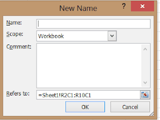
• Click on the Formula Tab and then  Click on ‘Define Name’.  The new name dialog box appears.
• Type the name you want to assign it to a range or constant. Ideally, it will be good practice to give a name which related to the value it refers to, though you can name it whatever you want.
• Select the scope of the defined name. You can choose for the full workbook or specified sheet.
• In the comment section, you can write something which describes your Named range or value. It is optional. It is better to write as it will be helpful when you refer this range after some time as you might forget what it refers to.
• ‘Refers to’ section you can enter a constant value or a range of cells. You can use browse icon to select the ranges or even you can manually enter it.
• Click Ok. You are done with defining the Names Range or Value.

Creating the Formulas using defined Named Ranges

We have already defined the range with a name. Now we will how to use that in the Excel functions or formulas. Use the functions or Formulas as usual. But instead of writing the range, type the name of that range you have defined. Below is the simple example which will give you better idea on how to use Named ranges in Excel Formulas.

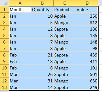
Below is the Sample Excel data which has Smartphone names and its price.

Here I have defined the range from B2 to B5 as ‘PriceRange’. Now for using this range in SUM function look as mentioned below.

=SUM(PriceRange).

Note: When you are using the named range in Excel Formula, as soon as you type first letter of your named range, you will see a drop down list which shows the named ranges. You can use that for easy to type the names.

Some times in Excel worksheet which we update frequently by adding new data to its columns and we need to reference the last value in a particular column. That is the value most frequently entered. We can achieve this combining two excel worksheet formulas COUNTA and INDEX. The source of this tips is John Walkenbach’s Excel 2010 Tips &Tricks book. To learn about find the last row using Excel VBA click here.

Below is the simple example with a excel worksheet which tracks the value of three funds in columns B to D. The data updates each and every month. The motto is to get the latest value for each fund and add the values of this.These value will be updated in the cells G2:G4.

The Excel formula used in G2,G3,G4 are as follows.
=INDEX(B:B,COUNTA(B:B))
=INDEX(C:C,COUNTA(C:C))
=INDEX(D:D,COUNTA(D:D))

Explanation on how this Excel Formula works: The COUNTA worksheet formula used above counts the number of non empty cells in the selected Column.Then this value is used as the second argument for INDEX worksheet function.  In the the first formula, in column B the last value is in row 6 hence COUNTA returns 6  and the INDEX function returns the 6th value in the column.

The above formula works on most of the situations. However, if the column has one or more empty cells interspersed(Empty cell in between the cells which has values), determining the last nonblank cells is challenging as COUNTA function doesnot count the empty cells.
The following array formula returns the content of the last non empty cell in the first 1000 rows of column C, even if column C contains blank cells.
=INDEX(C1:C1000,MAX(ROW(C1:C1000)*(C1:C1000<>””)))
Note: As this is a Array formula of Excel, you need to press Ctrl+Shift+Enter instead of just Enter. Otherwise it given wrong output.
You can change the formula to work with a column other than column C. To use a different column, change the column reference from C to whatever column you need. If the last non empty cell occurs in a row beyond row 1000, you need to change the two instances of 1000 to a desired row number. The fewer rows referenced in the formula, the faster the calculation speed.
To return the last non empty cell in a row, you need to use following excel array formula. It works similar to above formula, but finds last row instead of last column(In this example, row 1.
=INDEX(1:1,MAX(COLUMN(1:1)*(1:1<>””)))
to use this formula for a different row, change the the three 1:1 row references to correspond to the correct row number.

There is a direct Excel formula to count the number of characters in a cell. However, we sometimes come under a situation where we need to count a specific character in a cell or an occurrence of a substring in a cell.  Here are the steps to achieve these requirements.

Counting all the characters in a Cell

To count the number of characters in a cell, there is an Excel function called LEN. 

Syntax of LEN function

=LEN(text)

Examples for using Excel LEN function:

=LEN(A1)- it counts the number of character in Cell A1

=LEN(“Apple”)- counts the number of characters in the word “Apple”

Counting a specific characters in a Cell

To count a specific character in a cell, we need to use substitute and upper functions along with LEN function.

Example:

Let us consider we have a word “Apple” in Range A1 and we need to calculate the number of instances of “P”.

=LEN(A1)-LEN(SUBSTITUTE(UPPER(A1),”P”,””)) which returns 2.

This formula calculates the number of instances of “P” irrespective of case. If you want this formula to be case sensitive then formula becomes as mentioned below.

 =LEN(A1)-LEN(SUBSTITUTE(A1,”p”,””))

Explanation:

The Formula counts the total number of characters in the cell and subtracts the count of character of the cell excluding the character we need to calculate the count. Here SUBSTITUTE function is used to exclude the character “P”. SUBSTITUTE function is case sensitive; hence we have used “UPPER” function which makes all the characters in the cell to upper case in the first example. 

Counting the occurrences of a substring in a cell

Below example demonstrates on how to calculate the count of a specified string(more than a character) in a cell. 

=(LEN(A1)-LEN(SUBSTITUTE(UPPER(A1),UPPER(B1),””)))/LEN(B1)

In this example, the main string is in Cell A1 and the substring which we need to count is in cell B1.  For example. Cell A1 contains “Excel to Excel” and B1 contains “Excel” then the result is 2. The formula is not case sensitive. If you want to the formula to be case sensitive, then remove UPPER function which looks like below.

=(LEN(A1)-LEN(SUBSTITUTE(A1,B1,””)))/LEN(B1).