Tag: Excel Tips and Tricks

  • Different ways of using Single Criterion SUM function in Excel

    We have already seen the basic syntax and how to use single criteria SUM in Excel. In this post, we will see how use conditional sum based on difference scenarios. For detailed explanation on SUMIF function please read here.
    Examples for Using conditional sum Excel Function SUMIF: Below are the some of the Excel example based on different situations.
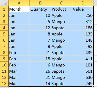
    Conditional sum Sample data
    Sample Data

    1. Summing only Negative OR Positive values using Excel SUMIF Function:

    The below formula will add the “difference” column values whichever is less than zero.
    =SUMIF(E2:E20,”
    Similarly you can add the values with positive value.
    =SUMIF(E2:E20,”>0″)

    Now if we want to find the total variations, we need to sum all negative values and positive values. Below is the formula to find total sum considering absolute values.
    =ABS(SUMIF(E2:E20,”0″) which returns 86. Here we did calculate the sum of both negative and positive values and then added these two making negative values absolute. 

    Note: The SUMIF function can use three arguments. However it is not mandatory to use third argument. If we omit the third argument, then Excel adds the values in the 1st argument when the criteria is met.

    2. Summing values based on a different Range:  For this we need to use the third argument of SUMIF functions.  As we know, first argument is the range which should be matched with the criteria(argument 2) and the third argument is the range which should be added when given criteria is met. Following SUMIF formula demonstrates the same.
    =SUMIF(E2:E20,”>0″,C2:C20) which returns 940. In this example, excel adds the “price” where the difference has positive value(Greater than Zero).
    3. Summing Values based on a text comparison: Some times we need to compare the text value of a range and then perform SUM.  Following are examples for the same.

    =SUMIF(A2:A20,”Apple”,C2:C20) which returns 444. This formula adds the range “Price” when “Data” Column has the text “Apple”.
    =SUMIF(A2:A20,”<>Apple”,C2:C20) which returns 997.This formula adds the range “Price” when “Data” Column does not contains text “Apple”.

    4. Summing Values based on a date Comparison: We can use Excel SUMIF formula to add the values based on given date criteria. Following is the example for the same.
    =SUMIF(B2:B20,”>=”&DATE(2013,1,7),C2:C20) which returns 790.
    =SUMIF(B2:B20,”>=”&TODAY(),C2:C20) which returns 217.

    Note: As you might have observed, we have used a expression as a second argument which is a criteria. The expression used in first example is DATE and in second it is Today().DATE function returns the date and Today function returns Todays date.  Also the comparison operator, enclosed in a quotation mark is concatenated using & operator with the result of the DATE or TODAY() function.

    Please share your thoughts or queries on these examples and also share any tips for using SUMIF function you might know in the comment section.0>0>

  • Using VLOOKUP on Excel-Explained with Syntax and Examples

    VLOOKUP functions of excel is very useful when you need to return a value from a table or a range of cells by looking up another value. VLOOKUP on excel can be used for finding the value in a range which are present in the other range in the same sheet or other sheet and other excel files. Let is quickly look into the syntax of vlookup function and examples on how to use VLOOKUP on Excel.  Do note than simple VLOOKUP function works with only single criteria. If you are looking for 2 or more criteria vlookup, the please refer my previous post multi criteria vlookup.

    Syntax of Excel VLOOKUP Function:

    = VLOOKUP( value, table_array, index_number, Typeoflookup )
    where
    Value: is the value to search for in the first column of the table_array or range of cells. Value can either a text or a numerical value.
    table_array: is the range of cells where you need to lookup for the value.
    index_number: is the column number in table_array from which the matching value must be returned. A index_number argument of 1 returns the value in the first column in table_array; a index_number of 2 returns the value in the second column in table_array, and so on.
    Typeoflookup: This is not mandatory. However this will chose between exact match and relative match.  If you use TRUE or if you omit this argument, then non exact match lookup will be performed. If this is set to FALSE, then vlookup does the exact match
    Note and Troubleshooting Tips on Excel:
    • If  “Typeoflookup” is either TRUE or omitted, the values in the first column of table_array must be placed in ascending sort order; otherwise, VLOOKUP might not return the correct value.
    • If “Typeoflookup” is FALSE, the values in the first column of table_array do not need to be sorted.
    • Excel vlookup returns #VALUE! if  “index_number” is less than 1 and returns  #REF! if the  “index_number”Greater than the number of columns in table_array. Also one more error value comes with VLOOKUP is #N/A. Excel returns #N/A when there is no exact match or the value you are matching in the range is not found.
    •  If there are two or more values in the first column of table_array that match the lookup_value, the first value found will be returned

    Example on Using VLOOKUP formula in Excel:

    Excel Examples
    Sample data

    Using vlookup with Exact match:

    Considering above sample data, if you need to lookup for the value “Banana” and fetch the Rating, use the formula given below.
    =VLOOKUP(“Banana”,A2:C6,3,FALSE) which returns C.

    Using vlookup with non Exact match:

    This is useful, when you need relative value. Say for example, your matching value based on the “% of commission” and you want to return the ratings. Here do not that, for using non exact match the first column of lookup range  must be placed in ascending sort order.
    =VLOOKUP(33%,B2:C6,2,TRUE) which returns C. Here first instance of nearby value is taken by the formula.

    Formatting the VLOOKUP on Excel using ISNA and IF functions:

    When there is no match found, excel returns #n/a.  This is will give problems when you need to use SUM function on the return value of returned value.To overcome this, we need to use ISERROR function. This very useful, if you are creating a template with VLOOKUP function.

    Examples:
    From the same above sample table, we will match Strawberry. The formula returns #n/a as the match is not found on the table.
    =IFERROR(VLOOKUP(“Strawberry”,A2:C6,3,FALSE),”Not Found”) which   returns “Not found”.
    The IFERROR functions syntax is =IFERROR(Value, value if error) where “value” is the data which needs to checked for error and “value for error” is the value to be returned incase of error.
    In above example we use VLOOKUP return data as value and “Not Found” used if the returned value is #N/A.
    IFERROR function was introduced in Excel 2007. Hence if you are using earlier version of Excel 2007, then you need to use IF function and ISERROR function of Excel. So the formula is as shown below.
    =IF(ISERROR(VLOOKUP(“Strawberry”,A1:C6,3,FALSE)),”Not Found”,VLOOKUP(“Strawberry”,A1:C6,3,FALSE))
    Note: Do not use this function unless you have earlier versions of excel as this will lead to calculation time. This is because for every time you use the function, excel needs to calculate vlookup twice. when range to lookup is more and number of instances of using this formula more, then excel will take really long time to calculate and return the right values.
    Please do share your feedback and tips which you know in the comment section below. If you need any specific support on Excel, then mention your query in comment section, I will try to answer your query.

    Video Tutorial for VLOOKUP

  • Using Excel Multiple condition COUNTIF function

    In my previous post, we have seen how to use single criteria Excel COUNTIF function. That works great  when you need to count a specific range of cells based on one condition.  Some times, there are situation we are required to count range of cells based on 2 or more conditions.  So let us have a quick look on the same.

    Excel Multi condition count function  with AND:

    The And criteria count function counts the cells if all the conditions are met.  The simple example for this is counting a range of cells which falls in between a numerical value. For example, counting cells that contains a value greater 0 and less than or equal to 20. Any cell that has positive value less than or equal to 20 will calculated in the Excel multi count with AND.For using this we need to use COUNTIF excel function or SUMPRODUCT function.

    Syntax of COUNTIFS function:

    =COUNTIFS(criteria_range1, criteria1, [criteria_range2, criteria2]…)

    Where
    criteria_range1:  Required. The first range in which to evaluate the associated criteria.
    criteria1 :  Required. The criteria in the form of a number, expression, cell reference, or text that define which cells will be counted. For example, criteria can be expressed as 32, “>32”, B4, “apples”, or “32”.
    criteria_range2, criteria2, …    Optional. Additional ranges and their associated criteria. Up to 127 range/criteria pairs are allowed.

    Note: COUNTIFS works only with Excel 2007 and higher versions. For using multiple condition count in earlier version of Excel we need to sumproduct.

    Syntax for using SUMPRODUCT function as multicondition count:

    As we have seen earlier, SUMPRODUCT function can be used to count range of cells based on multiple criteria.
    Example for using Multicondition count in Excel: Below the sample data.

    Counting only the sales of Apple for the month of Jan with value less than 250:
    1. Using countifs function: =COUNTIFS(A2:A13,”Jan”,C2:C13,”Apple”, D2:D13,”2. Using the SUMPRODUCT function: =SUMPRODUCT((A2:A13=”Jan”)*(C2:C13=”Apple”)*(D2:D13
    250>250>

    Using Multiple condition count with OR:

    To count cells by using an OR criteria, you should use multiple COUNTIFS functions.  For example, counting the number of instances of  8,6 and 5 in the range B2:B13.
    =COUNTIF(B2:B13,8)+COUNTIF(B2:B13,6)+COUNTIF(B2:B13,5)

    This can be achieved through COUNTIF function array formula of Excel.  The below Array formula returns the same result as that of above. As this is a array formula you need to enter the formula using Ctrl+Shift+Enter.
    =SUM(COUNTIF(B2:B13,{8,6,5})

    Note:  You need use flower bracket for 8,6,5 in the above example. 

  • Excel COUNTIF function Syntax with Examples

    The Excel COUNT and COUNTA formula is useful for the basic counting requirements. However, sometime you need to count a number of cells in a range which meets given criteria. To do this, COUNTIF formula is useful. So COUNTIF formula counts number of cells in a range based on the given criteria.
    Syntax of  Excel COUNTIF formula:
    COUNTIF(range, criteria)
    where
    range is range of cells which you need to count
    criteria is nothing but the condition on which the range should be calculated.

    Example for Excel COUNTIF Formula:
    Let us take below sample data and use countif function with different criteria.

    Excel Examples

    =COUNTIF(C2:C7,50) :- Counts the range with Value 50
    =COUNTIF(C2:C7,E1) : Counts the cells value equal to Range E1
    =COUNTIF(C2:C7,”>”&E1) : Counts the cells greater than value specified in the range E1
    =COUNTIF(D2:D7,”=COUNTIF(C2:C7,”*”): Counts the cells which contains text
    =COUNTIF(A2:A7,”Apple”): Counts only the cells with exact word Apple; not case sensitive
    =COUNTIF(A2:A7,”*Apple*”): Counts cells containing text Apple anywhere within the text
    =COUNTIF(A2:A7,”*E”) : Counts cells which cell content has the alphabet E in the last
    =COUNTIF(B2:B6,”>”&AVERAGE(B2:B6)) : counts the cells which are greater than average of the range.

    Using COUNTIF function with named ranges:  You can use Named Ranges in Excel countif function.  For doing this first we need to define the range.  Let us look into the above example and define Range A1:A7 as ” “Data”.

    Excel Tips

    Now we can use the names instead of writing the Ranges. The example for Countif function with named ranges.
    =COUNTIF(Data,”Mango”)
    Similarly we can use defined names to any range by naming that range. It is useful when we use complicated countif functions.0>

  • Using Absolute References in MS Excel

    When we apply a formula in Excel which refers to another range or cell, the cell or range reference can be wither relative or absolute.  The relative cell reference adjusts to its new location when the formula is copies and pasted in to new cell or range. An Absolute cell reference does not changes even when the formula is copy pasted elsewhere. An Absolute reference is specified with two doller($) signs. For example as mentioned below.
    Examples for Absolute references:
    =$C$10
    =SUM($A$1:$G$25)
    Examples for relative references:
    =C10
    =SUM(A1:S25)
    Normally when we use cell or range references which will be relative references. Excel by default creates relative cell references in formulas except when the formula includes cells in different worksheet or workbook.
    So where Absolute references are useful? I simple words, this is useful when we need to copy paste the formulas in different cells or ranges.

    Excel Examples

    The formula in the above example table D2 range which multiplies with quantity by the unit price is B2*C2. This formula uses the relative reference. Hence when we copy paste this formula to the next cell D3 it becomes B3*C3.
    If we use absolute reference in this formula that is instead of B2*C2, D2*$C$2, copying the formula to the below produces incorrect results. The formula in cell D3 is exactly the same as the formula in Cell D2 and returns the total for laptops and not desktops.
    Now let us use the same tablet to calculate sales tax.  The sales tax rate is stored in cell B7. Here formula in Cell E2 is D2*$B$7.

    The total is multiplied by the tax rate stored in cell B7. As this is constant for all the items, we need to give absolute references.  This reference do not change when we copy the cell.  When the same formula in E2 is pasted  to Cell E3, the formula becomes D3*$B$7. Here D3 is relative reference hence it changes but B7 remains same.