Tag: Excel Tips and Tricks

Excel do not provide a direct way to hide the contents of cells  without hiding entire row and column. However there is a indirect way to hide the content in the cell. Hiding cell content comes in handy, if you are using any template.

Steps to hide Cell Content in Excel

There various method to hide cell content in excel without hiding the row or column. These methods just make the content invisible to eye but we can refer this cell using the formulas.

Method 1:Use a special custom number format: Select the cell or cells to be hidden. Go to cell formatting. Select Custom and enter ;;;(three semi colons) in the Type field.

Method 2: Make the font color same as the cell’s background color.

Method 3: Add a shape to your worksheet and position it over the cells or cells to be hidden. Shape  color should have same color as the cell background and remove borders.

Method 4: Hiding cell content from  in the formula bar

All above method have one shortfall. That is even though content is not seen, it will be seen in the formula bar when cell is selected. To hide the the content from formula bar we need to hide formula bar or perform below mentioned steps .

• Select the cell or cells needs to be hidden.
• Right click on the cell and go to Format cells. Then click on Protection Tab in the Format Cells dialog box.
  Select the Hidden check box and Click OK.
• Choose Review->Changes->Protect Sheet.
• In the Protect sheet dialog box add a password if you need one. Click OK.

Note: When sheet is protected you can’t change any cells unless cell is unlocked. By Default, all the cells are locked. To unlock cell, select the cells you want to unlock. Go to Format cells and the go to Protection Tab. Uncheck the Locked check box.
Tip: Ctrl+1 is the shortcut key to reach format cells dialog box.

Hope this excel tutorial helps. Share your feedback in the comment section below.

There are many instances we need to split a text in a cell. The most common example for this is to split first name and last name. We can perform this using text to column feature of Excel. But if you want to create an template in Excel which requries you to split text in a cell, then you need to use either Excel function or Excel VBA.

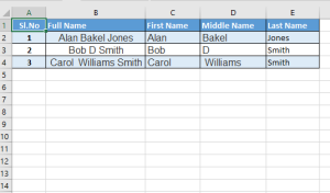
Luckily, Excel provides handy function through which we can extract desired word from the text.The formula uses various text functions to accomplish the task.Each of the techniques used here based on the ‘space’ between the names to identify where to split. So let us take an example of splitting full name into first, middle and last names.
Example:

Splitting a text in a cell using Excel Function

Extracting only First name from text using Excel Formula

For extracting first name from full name in cell, we can use left and find functions. So here is the way to how to do it.
Enter the formula in cell C2:

=LEFT(B2,FIND(” “,B2,1))

this will return Alan. similarly same formula in B3 will return Bob.
Syntax of Left function:LEFT(text,num_chars)
Where
Text is the text string that contains the characters you want to extract.
Num_char Specifies the number of characters you want LEFT to extract.
Note: 1.Num_chars must be greater than or equal to zero.2.If num_chars is greater than the length of text, LEFT returns all of text.3.If num_chars is omitted, it is assumed to be 1.
Syntax of Find Function: FIND(find_text,within_text,start_num)
Where
Find_text  is the text you want to find.
Within_text is the text containing the text you want to find.
Start_num  specifies the character at which to start the search. The first character in within_text is character number 1. If you omit start_num, it is assumed to be 1.

Extracting the Last Name from Text using Excel Formula

For extracting last name from a cell in excel, we need to take help of 3 functions. RIGHT, LEN and FIND function.
Eg: in cell E2 enter:

=RIGHT(B2,LEN(B2)-FIND(“#”,SUBSTITUTE(B2,” “,”#”,LEN(B2)-LEN(SUBSTITUTE(B2,” “,””)))))

will return Jones. Same formula for the rest the rows.
Syntax of Right function: RIGHT(text,num_chars)
Where Text:is the text string containing the characters you want to extract.
Num_chars:specifies the number of characters you want RIGHT to extract.
Above functions will not be able to handle any more than two names.If there is also a middle name, the last name formula will be incorrect.To solve the problem you have to use a much longer calculation.
Here is the function to solve this.
Enter =RIGHT(A4,LEN(A4)-FIND(“#”,SUBSTITUTE(A4,” “,”#”,LEN(A4)-LEN(SUBSTITUTE(A4,” “,””))))) in cell B4 will return Smith.  Here we have used additional function Substitute
Syntax of Substitute function:
SUBSTITUTE(text,old_text,new_text,instance_num)
Where
Text:   is the text or the reference to a cell containing text for which you want to substitute characters.
Old_text:   is the text you want to replace.
New_text: is the text you want to replace old_text with.
Instance_num:  specifies which occurrence of old_text you want to replace with new_text. If you specify instance_num, only that instance of old_text is replaced. Otherwise, every occurrence of old_text in text is changed to new_text.

Excel Function to extract middle name

Enter the following function in the cell E2:

 =RIGHT(B2,LEN(B2)-FIND(“#”,SUBSTITUTE(B2,” “,”#”,LEN(B2)-LEN(SUBSTITUTE(B2,” “,””)))))

You can use these functions in your excel sheets by making appropriate changes in the column and row numbers. If there is no middle name, the excel function will return #Value.

In the excel spreadsheet we will have formulas and data values.  There are some situation where we need to delete only values keeping formula in the sheet. Excel provides a solution for this. Here is a quick step by step way to select only values in a cell or only formulas in a cell.

It is very useful when you are working with excel templates. Excel templates normally will have cells with calculated fields. We just need to update the values. The Excel formulas will automatically generate the calculated cells.  The easiest way to do is just selecting the cells wityh only values and remove it. Now you can enter values in the blank cells. This will protect you from accidental removal of formulas.

This method of selecting only values in excel worksheet works on all the versions of Excel.  You can use this method to select only formulas or error values in a cell, last cell etc.

Step to retain only Values and deleting non formula cells

Below steps will guide you on how to select only values in a excel worksheet.

• Select the range where you want to delete only values, retaining formulas. If you want to delete all non formula value cells on the entire worksheet, then select any single cell.
• Chose Home->Editing->Find&Select->Go to Special. This will take you to the Go to Special dialog box.
• In the Go To Special dialog box, select the Constants option and then select Numbers.
• Click OK. Now only nonformula numeric cells are selected.
• Press Delete to delete the values.

Note:

1. If you need to delete the value cells on a regular basis, then you can specify a name for the input cells. This can be achieved through defining the names to range. After completing Step 4 choose formula ->Defined Names-> Define Name to display the new Name box. Enter a name for the selected cells. Click OK to close the New Name Dialog box and create the name. After naming the input cells, you can select the named cells directly by using the Name box- the drop down list to the left of the Formula bar. Then press delete and you are done.
2. Shortcut key to reach Goto Special dialog box is Ctrl+G and Alt+S.

Excel can work with Time very easily. With Time excel can perform many formatting and calculations based time. Let us have a look into this. In this excel tips we will learn few tasks we can perform on Excel with time formats.

Typing Time in Excel Worksheet

When time is entered into worksheet it should be entered with a colon between the hour and the minutes, such as 12:30, rather than 12.30.Excel can cope with either the 24hour system or the am/pm system.To use the am/pm system you must enter the am or pm after the time.You must leave a space between the number and the text.
Example for writing Time in 24 hour format:
01:30, 2:30, 20:10, 23:30 etc
Example for writing Time in AM/PM format:
1:30 AM, 2:30 AM, 8:10 PM, 11:30 PM etc

Calculation of Time differences in Excel

:
You can add or subtract the two times to get know the length of the time or add the two time times to get total time.
Example for Subtracting two Times in Excel:

Now you can use formula like this to find difference between the two times.Enter  =A2-B2 in the required result cell. You will get 1:00. And the second one will give you 9:00(A3-B3).
Example for Adding two times in Excel:

Consider above table. Adding is very easy. Enter formula =A2+B2 which returns 04:00 and the second row will return 25:00:00. Some time it just returns 1 hours. This is because of the cell formatting. Let us look into the   time formatting.

Formatting of Time in Excel:
Considering above example second row 3. Sum goes beyond 24 hours. The general time format will show only the time excluding the number of days. For correcting this,  easiest way is to opt for Custome formatting.
Applying Custom Formatting to Time to show exact value:

• Click on the cell which needs the format.
• Choose the Format menu.
• Choose Cells.
• Click the Number tag at the top right.
• Choose Custom.
• Click inside the Type: box.
• Type [hh]:mm as the format.
• Click OK to confirm.hoose Custom.
• Click inside the Type: box.
• Type [hh]:mm as the format.
• Click OK to confirm.