Tag: VLOOKUP Tips and tricks

  • VLOOKUP Tips and Tricks- EXCEL Tutorial

    VLOOKUP in Excel is one of the most powerful and useful function which helps to save our time on many occasions. Some of the situations where VLOOKUP comes in handy are fetching data from other tables, matching two different series, creating one list from multiple related lists etc.  This post is not on how to use VLOOKUP in excel. This post is all about some of the useful tricks which is helpful to use VLOOKUP in excel in an effective way.

    VLOOKUP Tips and Tricks

    1. Using the $ for lookup value and lookup range

    When you are copy and pasting the VLOOKUP in excel to different cells, you might have noticed errors. This happens because while you are pasting the formula, range changes. To avoid this, you can use the absolute range or value. To make the value absolute you should use $ symbol.

    For example, consider an example.

    =vlookup(a2,c2:d5,2,false)

    The above formula is there in cell G2. If you copy and paste the formula in G3, the formula changes to  =vlookup(A3,C3:D6,2,false). If you copy the formula in the cell H2, then formula changes to =vlookup(B3,D2:E6,2,false). To avoid this, we can use $ or it is called absolute reference.  $ makes the row or column absolute. If you use before column name then, the column will become absolute. If you use before row number, then row number will become absolute.  Likewise, if you use $ before column and row number, then both column and row will become absolute. There are different ways to use absolute references in excel depending on the situations. Let’s learn more on this with the same example mentioned above.

    Scenario 1: =VLOOKUP($A$2,$C$3:$D$6,2,false)- In this case, wherever you copy this formula, it will lookup for the value in cell A2 in range C3 to D5 of the active sheet.

    Scenario 2: =VLOOKUP($A2,$C$3:$D$6,2,false)- Here lookup range and column of the lookup value remains constant. However, row number changes depending on where you paste the formula. This can be used when lookup value in there in column A.

    Similarly, you can use the absolute reference for the range as well.

     2. Understanding error values of VLOOKUP

    Majorly, while using VLOOKUP in excel 3 errors values come out. They are #NAME, #N/A and #VALUE.

    What is this means? How to fix it.

    #NAME error in VLOOKUP:  If you get #NAME error, then it means that there is a spelling error in the formula. Please check the syntax and fix it.

    #VALUE error in VLOOKUP: This commonly appears when the column index number is less than the range you have selected. For example, if you have selected the column index number as 5 wherein the range has only 4 columns this error will come. Please check the lookup range and column index to fix this. Another possible cause might be lookup value length is more than 255 characters.   

    #N/A error in VLOOKUP: This is not necessarily an error.  This means that the value you are looking for in the range is not available.  The things you should check are

    • Is lookup value is correct?
    • Are any blank spaces before or after the lookup value? If yes use trim or clean functions to remove spaces.
    • Have you had selected the range where the first column has the value you are looking for lookup value? -If no, select the range such way that, a column on which you are looking for the lookup value should be the first column in the range. The format of the lookup value and lookup range should be same.

    3.  Working with errors

    When the lookup value is not available in lookup range, VLOOKUP gives error #N/A. If you are using the further calculation based on the resulting result, then that also shows as #N/A. To hide this or to make cells look cleaner you can use the formula IFERROR with VLOOKUP. It will look like this IFERROR(VLOOKUP(….), “VALUE to be WRITTEN IN CASE OF ERROR”)).

    4. ROW and COLUMN VLOOKUP or multi conditional VLOOKUP

    We already know that VLOOKUP in EXCEL can be used for fetching data based on the lookup value. But how to use multi conditional VLOOKUP in EXCEL. This means that the resulting data should be matched with both row and column. This can be done with help of MATCH function with VLOOKUP. You need to replace, column index or 3rd argument of VLOOKUP with match function.

    Example for the same is as mentioned below.

    =VLOOKUP($A9,$A$1:$D$6,MATCH(B$8,$B$1:$D$1,1)+1,FALSE)

    You can read more on this here.

    5. Partial match with VLOOKUP

    Making forth argument of VLOOKUP as TRUE will perform partial match. But it has many restrictions. Instead, you can use wildcard characters in VLOOKUP function to perform partial match. Basic wildcard charecter for partial match are,

    “*”: Find any number of characters after or before text. For example, you can use “Te*” to match the text “Text” from a list or *Te to match the text “Forte”.

    “?”: Use a question mark to replace with a character. For example, you can use “?aste” to lookup for the text “Waste” or “Taste”.

    These are the basic yet effective VLOOKUP tips to make your work easier and use this function more effeciently. If you have any queries do write in the comment section below.
  • Using VLOOKUP on Excel-Explained with Syntax and Examples

    VLOOKUP functions of excel is very useful when you need to return a value from a table or a range of cells by looking up another value. VLOOKUP on excel can be used for finding the value in a range which are present in the other range in the same sheet or other sheet and other excel files. Let is quickly look into the syntax of vlookup function and examples on how to use VLOOKUP on Excel.  Do note than simple VLOOKUP function works with only single criteria. If you are looking for 2 or more criteria vlookup, the please refer my previous post multi criteria vlookup.

    Syntax of Excel VLOOKUP Function:

    = VLOOKUP( value, table_array, index_number, Typeoflookup )
    where
    Value: is the value to search for in the first column of the table_array or range of cells. Value can either a text or a numerical value.
    table_array: is the range of cells where you need to lookup for the value.
    index_number: is the column number in table_array from which the matching value must be returned. A index_number argument of 1 returns the value in the first column in table_array; a index_number of 2 returns the value in the second column in table_array, and so on.
    Typeoflookup: This is not mandatory. However this will chose between exact match and relative match.  If you use TRUE or if you omit this argument, then non exact match lookup will be performed. If this is set to FALSE, then vlookup does the exact match
    Note and Troubleshooting Tips on Excel:
    • If  “Typeoflookup” is either TRUE or omitted, the values in the first column of table_array must be placed in ascending sort order; otherwise, VLOOKUP might not return the correct value.
    • If “Typeoflookup” is FALSE, the values in the first column of table_array do not need to be sorted.
    • Excel vlookup returns #VALUE! if  “index_number” is less than 1 and returns  #REF! if the  “index_number”Greater than the number of columns in table_array. Also one more error value comes with VLOOKUP is #N/A. Excel returns #N/A when there is no exact match or the value you are matching in the range is not found.
    •  If there are two or more values in the first column of table_array that match the lookup_value, the first value found will be returned

    Example on Using VLOOKUP formula in Excel:

    Excel Examples
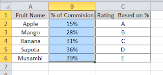
    Sample data

    Using vlookup with Exact match:

    Considering above sample data, if you need to lookup for the value “Banana” and fetch the Rating, use the formula given below.
    =VLOOKUP(“Banana”,A2:C6,3,FALSE) which returns C.

    Using vlookup with non Exact match:

    This is useful, when you need relative value. Say for example, your matching value based on the “% of commission” and you want to return the ratings. Here do not that, for using non exact match the first column of lookup range  must be placed in ascending sort order.
    =VLOOKUP(33%,B2:C6,2,TRUE) which returns C. Here first instance of nearby value is taken by the formula.

    Formatting the VLOOKUP on Excel using ISNA and IF functions:

    When there is no match found, excel returns #n/a.  This is will give problems when you need to use SUM function on the return value of returned value.To overcome this, we need to use ISERROR function. This very useful, if you are creating a template with VLOOKUP function.

    Examples:
    From the same above sample table, we will match Strawberry. The formula returns #n/a as the match is not found on the table.
    =IFERROR(VLOOKUP(“Strawberry”,A2:C6,3,FALSE),”Not Found”) which   returns “Not found”.
    The IFERROR functions syntax is =IFERROR(Value, value if error) where “value” is the data which needs to checked for error and “value for error” is the value to be returned incase of error.
    In above example we use VLOOKUP return data as value and “Not Found” used if the returned value is #N/A.
    IFERROR function was introduced in Excel 2007. Hence if you are using earlier version of Excel 2007, then you need to use IF function and ISERROR function of Excel. So the formula is as shown below.
    =IF(ISERROR(VLOOKUP(“Strawberry”,A1:C6,3,FALSE)),”Not Found”,VLOOKUP(“Strawberry”,A1:C6,3,FALSE))
    Note: Do not use this function unless you have earlier versions of excel as this will lead to calculation time. This is because for every time you use the function, excel needs to calculate vlookup twice. when range to lookup is more and number of instances of using this formula more, then excel will take really long time to calculate and return the right values.
    Please do share your feedback and tips which you know in the comment section below. If you need any specific support on Excel, then mention your query in comment section, I will try to answer your query.

    Video Tutorial for VLOOKUP