Category: Excel Basics

  • How to Round a Number to Closest ten in Excel

    Rounding a number in Excel is very easy. There are situation wherein we need to round a number to closest 10 or 100. For example, if we have a number 115 then 120, if we have 112 then 110. For this there is a dedicated function in Excel called MROUND which comes useful for such scenario. Let us learn more about the function MROUND in Excel.

    Syntax of Excel MROUND function

    MROUND(number, multiple)

    Where,

    • Number Required. The value to round.
    • Multiple Required. The multiple to which you want to round number.

    Note: MROUND rounds up, away from zero, if the remainder of dividing number by multiple is greater than or equal to half the value of multiple.

    Example:

    Below are the few useful examples of MROUND in Excel.

    1. Rounding a number to multiples of 10

    =MROUND(112, 10) Rounds 112 to the nearest multiple of 10 which will return 110

    =MROUND(116, 10) Rounds 116 to the nearest multiple of 10 which will return 120

    2. Rounding a number to multiples of 5

    =MROUND(112, 5) Rounds 112 to the nearest multiple of 5 which will return 110.

    =MROUND(116, 5) Rounds 116 to the nearest multiple of 5 which will return 115.

    =MROUND(118, 5) Rounds 118 to the nearest multiple of 5 which will return 120.

    There are other two Excel function which are very similar to this function but with slight change on the functionality.

    1. CEILING(number,significance)

    This will Returns number rounded up, away from zero, to the nearest multiple of significance. For example

    CEILING(112,5) will return 115

    CEILING(112,10) will return 120

    CEILING(115,5) will return 120.

    2.FLOOR(number,significance)

    This will Rounds number down, toward zero, to the nearest multiple of significance.  For example,

    FLOOR(112,5) will return 110

    CEILING(115,10) will return 110.

    So in summary, MROUND Excel function is useful when we need to round number up or down to the nearest multiple. Whereas if you want roundup decimals then ROUNDUP function is useful. For rounding down decimal ROUNDDOWN excel function is useful. Depending on the requirements, these Excel functions will help us to save our time.
  • How to unhide first row or Column in a Excel Worksheet

    At times, in Excel worksheet the first row(Row 1) or first column(column A) doesnot show up. It is tricky to unhide  the first row or column as there is no easy way to do it. Based on the situation, you need to apply different method to access the first row or column. So here is the quick possible reasons for hidden first row or first column.
    Reasons and Solutions  for Hidden First Row or First Column

    Hidden First row or Column
    1. The row or column is hidden: Most of the time we might have hidden that row or column. Unhiding first row or column is as said earlier is not easy. For doing so, simplest method is to select whole sheet and right click and select Unhide.
    2. Another possibility is freezed columns or rows: If a excel worksheet has freezed row or columns, then also you will not be able to access some rows and column. Try Unfreezing by going to View->Freeze Panels.
    3. Row or Column size reduced to very small: Some excel worksheet which we get has very small sized row or column which we cannot see the row or column. In this scenario, select entire worksheet by selecting entire row. Right click and increase row height. If it is column, then select columns and enter higher column width.
    Other solutions for unhiding first row or column:
    1. In the Name Box next to the formula bar, type A1 and then press ENTER.
    2. On the Home tab, in the Editing group, click Find & Select, and then click Go To. In the Reference box, type A1 and then click OK.
    Hope these steps helped you to unhide your excel worksheet first row or column. Still if you have any problems share it in the comment section below.
  • How to Remove spaces from a cell in Excel

    In today excel tip let us discuss on how to remove leading space and trailing space in a cell of Excel worksheet.  By default there are three excel functions which are very useful in removing the space in a cell. The Excel function we are going to use cleanup the cell are CLEAN, TRIM and SUBSTITUTE function.

    TRIM Excel Worksheet Function:
    The TRIM function is used to remove spaces from a text excluding the one which is there in between two words. The syntax of TRIM function is as follows.
    TRIM(text)
    Examples:
    TRIM(A17) which removes the spaces in the starting of the text and end of the text.
    CLEAN Excel Worksheet Function:
    The CLEAN worksheet function removes all the non printable characters from the text. In real time, we can use CLEAN function for data which is exported from the other applications which contains characters that may not print with your operating system. The syntax of CLEAN function is as follows.
    =CLEAN(text)
    If you want to remove non printable characters as well as space, then you need to first use CLEAN function and then use the TRIM function.
    SUBSTITUTE Excel Worksheet Function
    The substitute function helps you to replace old text with new text. The syntax for substitute function is as follows.
    SUBSTITUTE(text,old_text,new_text,instance_num)
    Text     is the text or the reference to a cell containing text for which you want to substitute characters.
    Old_text     is the text you want to replace.
    New_text     is the text you want to replace old_text with.
    Instance_num     specifies which occurrence of old_text you want to replace with new_text. If you specify instance_num, only that instance of old_text is replaced. Otherwise, every occurrence of old_text in text is changed to new_text.
    As you could has assumed, now we can use this formula to replace blank with non blank. Look for the example below.
    =SUBSTITUTE(A1,” “,””)
  • Maximum and Minimum Worksheet Functions in Excel

    There are many situation where we need to find the maximum and minimum in a range. Like many other worksheet functions, finding the maximum and minimum also there is a direct functions available. Let us have a quick look into the maximum and minimum excel worksheet functions.
    Finding Maximum in a range using the Excel worksheet function:
    As said earlier, we need to use max function to get the maximum in a range.
    The syntax of max worksheet function is
    =max(number1, number 2, number 3…….Number n)
    where number1, number 2, number 3…….Number in which we need to find the maximum value.
    Examples on MAX excel function:
    =max(23,18, 51, 49)  this will return 51
    =max(A1:A4)
    Finding Minimum in a range using the Excel worksheet function:
    The syntax of MIN function in excel is
    =min(number1, number 2, number 3…….Number n)
    Where number1, number 2, number 3…….Number n Number in which we need to find the maximum value.
    Examples on Excel MIN function:
    =min(23,18, 51, 49)  this will return 18.
    =min(A1:A4)
    We have seen how to find the simple minimum and maximum using the excel functions. But at times we need to find max in a range with a criteria. There is a conditional max function available.
    For finding the conditional max in range we need to use DMAX function.
    The syntax for DMAX is
    DMAX( database, field, criteria )
    Where
    database is the range of cells that you want to apply the criteria against.
    field is the column to find the largest number in. You can either specify the numerical position of the column in the list or the column label in double quotation marks.
    criteria is the range of cells that contains your criteria.
  • Handling Error Displays in Excel Formulas

    Sometimes when we use a formula in an Excel worksheet it returns error values such as #N/A, #REF! or #DIV/0!. In some situations we want to know whether the formula returns error values. In some scenarios we do not want to show error values. For example when we create a templates in excel with VLOOKUP, then there will be a error values. To make it look neat, removing error values is an good idea.

    To hide or not to display error values, there primary ISERROR function with IF or direct IFERROR function in Excel 2007 or later will be useful. So let us see simple example so that, you will understand better.

    Different Excel Formulas to Hide Error Values

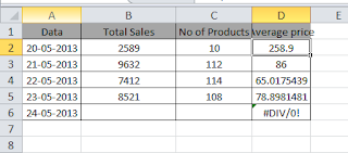
    Below is the sample data and based on this table we will try different ways to hide error messages.

    IF and ISERROR examples
    In the above data, Column D calculates the average price of the products. For this we have used =B2/C2 formula.
    Method 1: Using ISERROR Function with IF condition 
    As you can see from the above table, the formula returns an error if the cells used in the calculation are empty. If you want to hide that error value then use IF function to check an error value using along with ISERROR function. Then the formula becomes
    =if(error(B2/C2),””,B2/C2)
    How it works:
    ISERROR function retunrs true if the argument evaluates to an error.  Then IF function retunrs an empty string otherwise IF function returns the calculated value. You can use this logic with any formula which returns error value such as division, VLOOKUP in Excel etc.
    Using the IFERROR Function
    This formula does the same thing as above. But here it it formula evaluates only once.  This will help you to make your worksheet faster.
    The Formula becomes as below.
    =IFERROR(B2/C2,””)
    Do note that, IFERROR function is first introduced in Excel 2007. So previous versions of excel do not support this function.