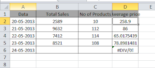
Sometimes when we use a formula in an Excel worksheet it returns error values such as #N/A, #REF! or #DIV/0!. In some situations we want to know whether the formula returns error values. In some scenarios we do not want to show error values. For example when we create a templates in excel with VLOOKUP, then there will be a error values. To make it look neat, removing error values is an good idea.
To hide or not to display error values, there primary ISERROR function with IF or direct IFERROR function in Excel 2007 or later will be useful. So let us see simple example so that, you will understand better.
Different Excel Formulas to Hide Error Values
Below is the sample data and based on this table we will try different ways to hide error messages.
In the above data, Column D calculates the average price of the products. For this we have used =B2/C2 formula.
Method 1: Using ISERROR Function with IF condition
As you can see from the above table, the formula returns an error if the cells used in the calculation are empty. If you want to hide that error value then use IF function to check an error value using along with ISERROR function. Then the formula becomes
=if(error(B2/C2),””,B2/C2)
How it works:
ISERROR function retunrs true if the argument evaluates to an error. Then IF function retunrs an empty string otherwise IF function returns the calculated value. You can use this logic with any formula which returns error value such as division, VLOOKUP in Excel etc.
Using the IFERROR Function
This formula does the same thing as above. But here it it formula evaluates only once. This will help you to make your worksheet faster.
The Formula becomes as below.
=IFERROR(B2/C2,””)
Do note that, IFERROR function is first introduced in Excel 2007. So previous versions of excel do not support this function.

Leave a Reply