Category: Excel Tips

Excel tutor on formulas, tips and tricks and VBA.

  • Excel If Function – Syntax And Examples

    Excel IF function is one of my favorite function in Excel. It is very useful and very simple to use. It does wonders when you want to create some complicated excel Formulas. You can extend the functionalities of IF function by nesting it or using along with other Excel Functions such as VLOOKUP, AND, OR etc.
    How Excel IF Function Works?
    Excel IF Function  checks for a condition(Criteria) and returns a value if the condition is met or returns another value if the criteria is not met. The criteria can be anything such as comparison, text check or error check etc. You can use nested IF functions upto 98 times in a excel worksheet.

    Syntax of Excel IF Function

    =if(condition, value if the condition is met, value if condition is not met)

    Examples:
    =if(A1>10, “Greater Than 10”, “Less than 10”)

    The Above IF formula returns Greater than 10 if the cell A1 has the value greater than 10 else returns Less than 10.

    Using IF function with AND

    As said earlier, you can use AND function inside IF  while you want a value to be written provides multi conditions were met. AND function returns TRUE if and only if  all the conditions are TRUE.For example, you have a value in cell A1. You want to check whether the number is in between 10 to 15. You can use the IF function as mentioned below.
    IF(AND(A1>10,A1

    Using IF function with OR

    IF and OR is used when you want to check any of the conditions is met. The OR Function returns true if any of the condition is met. For example you have want to check out of range if the number in cell A1 is less than  0 or greater than 100. You can use IF function with OR to calculate this as mentioned below.
    IF(OR(A1>100,A1

    Using Nested IF Function

    Using IF functions inside another IF function is called as nested IF functions. It is useful when you want to dig into the more detailed checks. For example you want to check if the number you have entered is a negative or positive in the cell A1.  First we need to check whether the entered value is number. If it is a number, then we need to check whether it 0. Then we need to check whether it is greater than 0 or less than 0 to find out the value entered is positive or negative. The nested IF function in Excel looks like as mentioned below.
    =IF(ISNUMBER(A1), IF(A1=0,”NIL”,IF(A1>0,”Positive Number”,”Negative Number”)),”It is not a Number”)
    The above uses ISNUMBER function to check for the whether the entered value is number or not.
    To learn how to use IF function with vlookup read my post on how to do vlookup on different ranges based on criteria.

  • Hiding or Unhiding Rows and Columns in Excel using Buttons

    Have you seen a excel spreadsheets with + or – symbols which on clicking unhides or hides rows and columns?  You might think that, it is done using Excel VBA. But this is not done by any VBA code. It is a simple grouping features of Excel. It is very useful when you want to display only the summary and show details with single button click. Lets start learning how to group and ungroup in Excel.
    For example you might have data which contains datewise data along with Weekly summary. You can show only the summary and provide the option to user to view the details using the + or – buttons

    Steps to Group Rows or Columns in Excel

    Step 1: Select the cells you want to group it. You can choose rows or columns according to your requirement. In this example i am selecting the rows from A2 to A5.
    Step 2: Go to Data and click on Group and select Group once again.  Your selected rows or columns are grouped.
    Step 3: There will be  + sign when your details are grouped and showing only summary. Where clicking on + sign will expand the group

    Steps to Ungroup rows or Columns

    Step1: Select the rows or columns you have Group enabled.
    Step2: Go to Data and select Ungroup and choose Ungroup.
    Step3: The Group is removed.

    As mentioned earlier, grouping in excel is very useful for presenting the data in good manner. Advantages of grouping is it shows the summary and it required, the all the details are also there. Unlike simple row/column hiding, in grouping you will will have symbol which indicates that, there is a grouping.

    Hope this Excel tips is useful. If you find this guide useful, then please share it with your friends. Any queries and support needed, then leave a comment below.

  • Type Rupee Symbol in Excel 2010

    Ever since the introduction of Rupee symbol, usage is also increased. When we type, we would like to use Rupee symbol rather than Rs. I have already made a tutorial on how to type rupee symbol in keyboard windows. That post is useful if you want to write rupee symbol in MS word or blogging platforms such as blogger, WordPress etc.

    Recommended Reading:

    Type INR Symbol in Word

    Conditional VLOOKUP in EXCEL

    However, if you want to use Rupee symbol in  Excel 2010, there is a simple way than that. You can easily insert rupee symbol in excel spreadsheet by choosing the currency symbol rupee in the format tab. There is no need to install any update or any change of keyboard layout if you want to use Rupee symbol in excel 2010. Just follow the steps given below.

    Steps to Insert Rupee Symbol in Excel Worksheets

    Step1: Enter the values as desired.
    Step2: Select the cells which you want to insert rupee cell.
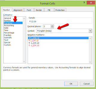
    Step 3: Right click and go to format cells.
    Step 4: Select Currency from the category.  In the symbol drop down, scroll down till you see ₹ English (India).

    Step 5: Click Ok. Your cells are converted into currency and it shows along with the rupee symbol.
    Hope this help on inserting rupee symbol in excel. If you have any difficulties, please share in the comment section.

    Note:
    • If you are not able to find English (India) under the symbol, then you need to install the keyboard layout and make it as default.
    • If you want to enter Rupee symbol while entering in the cell, you can use shortcut key Ctrl+Alt+$(4) combination.
    • If you want to update many rows, then you need to use the method which I have mentioned above.
    • This method of typing Rupee symbol works with Excel 2016 also.

    Video guide on how to use Rupee Symbol in EXCEL

  • Using Dynamic Named Formula in Excel

    It is a useful concept which saves you a lot of time when you are working with multiple formulas in bigger data range.  The Dynamic named Ranges means the range that isn’t fixed and it can be increased or decreased automatically as per the size of the data. This can be achieved using named ranges feature of Excel without using VBA macros. We will understand this better with a simple example.

    Using Named Formula Ranges in Excel

    Below is the sample data of a sales shop which continuously updates on daily basis.
    Excel Tips and Tricks Examples
    You want to create a name for the data in Column A without referring to empty cells. In simple words, reference to the Dateofpurchase changes every day as you add a new transaction.   In this scenario you can create a dynamic named formula that changes automatically as you enter new data or delete existing data.

    Steps to Create Dynamic Named Formula

    1. Goto Formulas->Defined names-Define Name to display the New Name Dialog box.
    2. Enter DateofPurchase in the Named Field.
    3. Enter the following formula in the  Refers to Field and Click Ok to Close Name Dialog box.

    =OFFSET(Sheet1!$A$2,0,0,COUNTA(Sheet1!$A:$A),1)

    Dynamic Named Formula Creation
    The above step creates a named Formula that uses the excel OFFSET and COUNTA functions to return a range that changes based on the number of non empty cells in column A.To test this let us use a simple COUNTA function

    =COUNTA(Date_Of_Purchase)  

    As you can see, the value changes when you add a new transaction or delete a transaction. This is very useful when you work on large data. Because it uses dynamic memeory allocation, it increases the calculation speed of the formulas. You can see actual difference when you use this with multiple VLOOKUP formula on a large Data range.
    Note:
    The Above shown method works only when you have non empty data range. That is, the range should not contain blanks in between.

  • Handling Error Displays in Excel Formulas

    Sometimes when we use a formula in an Excel worksheet it returns error values such as #N/A, #REF! or #DIV/0!. In some situations we want to know whether the formula returns error values. In some scenarios we do not want to show error values. For example when we create a templates in excel with VLOOKUP, then there will be a error values. To make it look neat, removing error values is an good idea.

    To hide or not to display error values, there primary ISERROR function with IF or direct IFERROR function in Excel 2007 or later will be useful. So let us see simple example so that, you will understand better.

    Different Excel Formulas to Hide Error Values

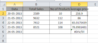
    Below is the sample data and based on this table we will try different ways to hide error messages.

    IF and ISERROR examples
    In the above data, Column D calculates the average price of the products. For this we have used =B2/C2 formula.
    Method 1: Using ISERROR Function with IF condition 
    As you can see from the above table, the formula returns an error if the cells used in the calculation are empty. If you want to hide that error value then use IF function to check an error value using along with ISERROR function. Then the formula becomes
    =if(error(B2/C2),””,B2/C2)
    How it works:
    ISERROR function retunrs true if the argument evaluates to an error.  Then IF function retunrs an empty string otherwise IF function returns the calculated value. You can use this logic with any formula which returns error value such as division, VLOOKUP in Excel etc.
    Using the IFERROR Function
    This formula does the same thing as above. But here it it formula evaluates only once.  This will help you to make your worksheet faster.
    The Formula becomes as below.
    =IFERROR(B2/C2,””)
    Do note that, IFERROR function is first introduced in Excel 2007. So previous versions of excel do not support this function.